Curs festiv

2006

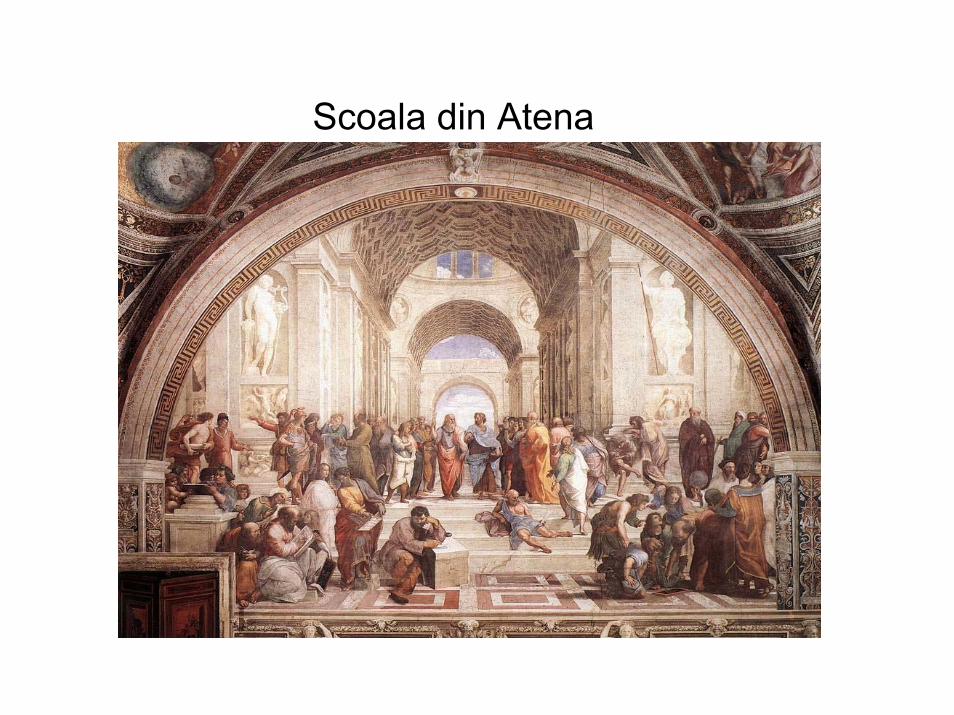
Scoala din Atena

PROFESORI CA PLATON SI ARISTOTEL

EUCLID SI PITAGORA

• IN EVUL MEDIU

IN EVUL MEDIU (CAM 1350)

SORBONA IN SECOLUL XVII

SORBONA IN ZILELE NOASTRE

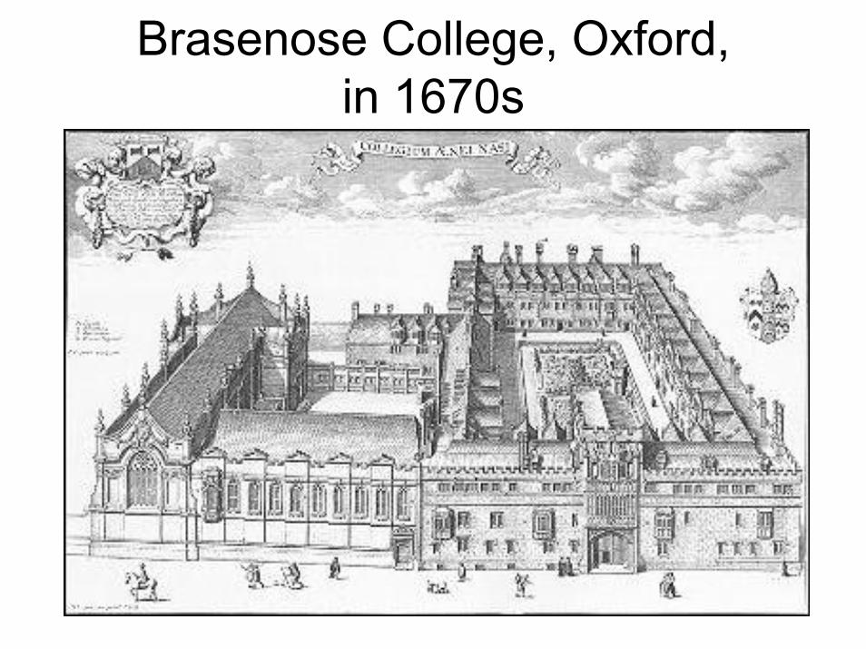
Brasenose College, Oxford, in 1670s

ALTA EPOCA, ALTI PROFESORIMichael Faraday

LABORATORUL LUI FARADAY

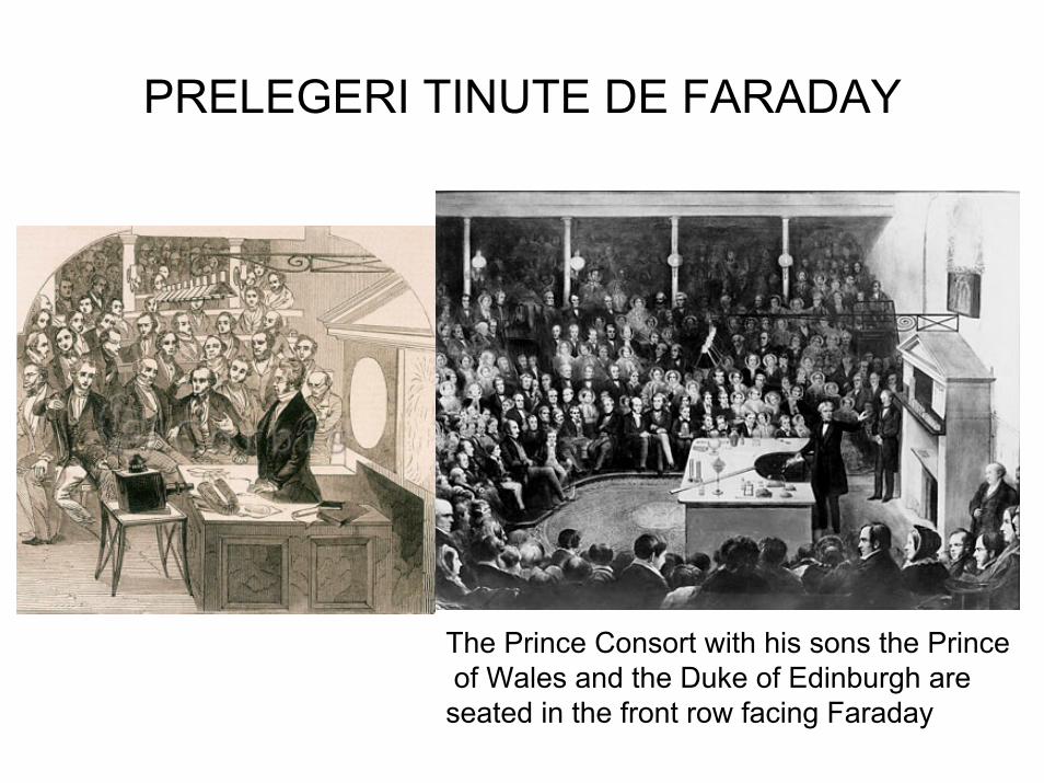
PRELEGERI TINUTE DE FARADAY

The Prince Consort with his sons the Princeof Wales and the Duke of Edinburgh are

seated in the front row facing Faraday

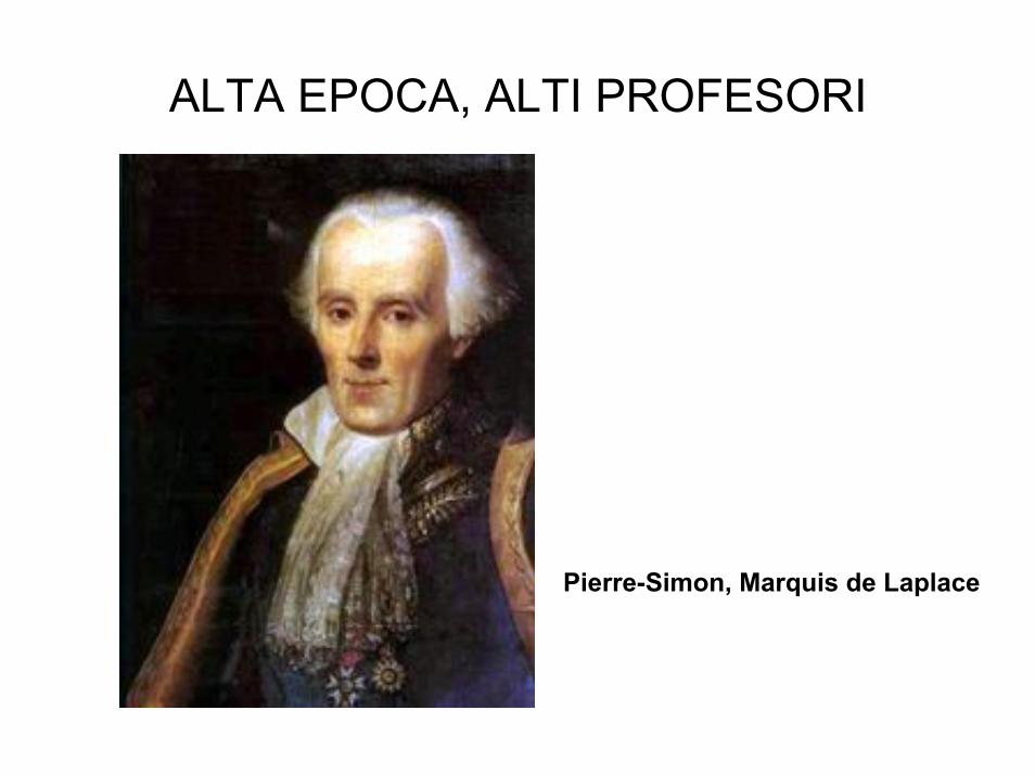
ALTA EPOCA, ALTI PROFESORI

Pierre-Simon, Marquis de Laplace

FOURIER, CEL CE A ADUS ATATEA “NECAZURI”

HEINRICH HERTZ

MAXWELL CU ECUATIILE SALE

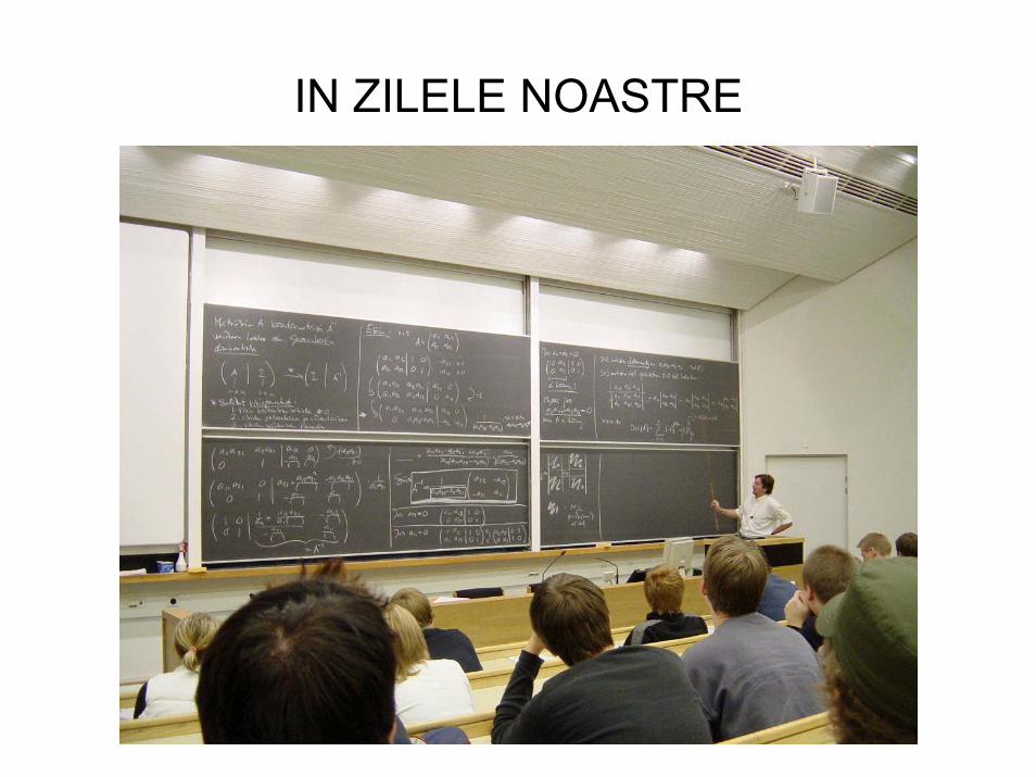
IN ZILELE NOASTRE

DIRAC, CEL CU IMPULSUL UNITAR

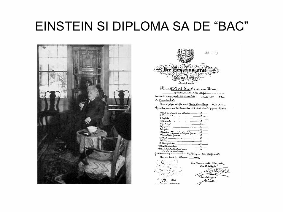
EINSTEIN SI DIPLOMA SA DE “BAC”

SHANNON SI KOTELNIKOV

CATEVA PERSONALITATI DIN ROMANIA

Augustin Maior ( 1882 - 1963 ) Iancu Constantinescu ( 1884 - 1963 )Sergiu Condrea ( 1900 - 1986 ) Tudor Tanasescu ( 1901 -1961 ) Remus Radulet (1904 – 1984 )Alexandru Rogojan ()

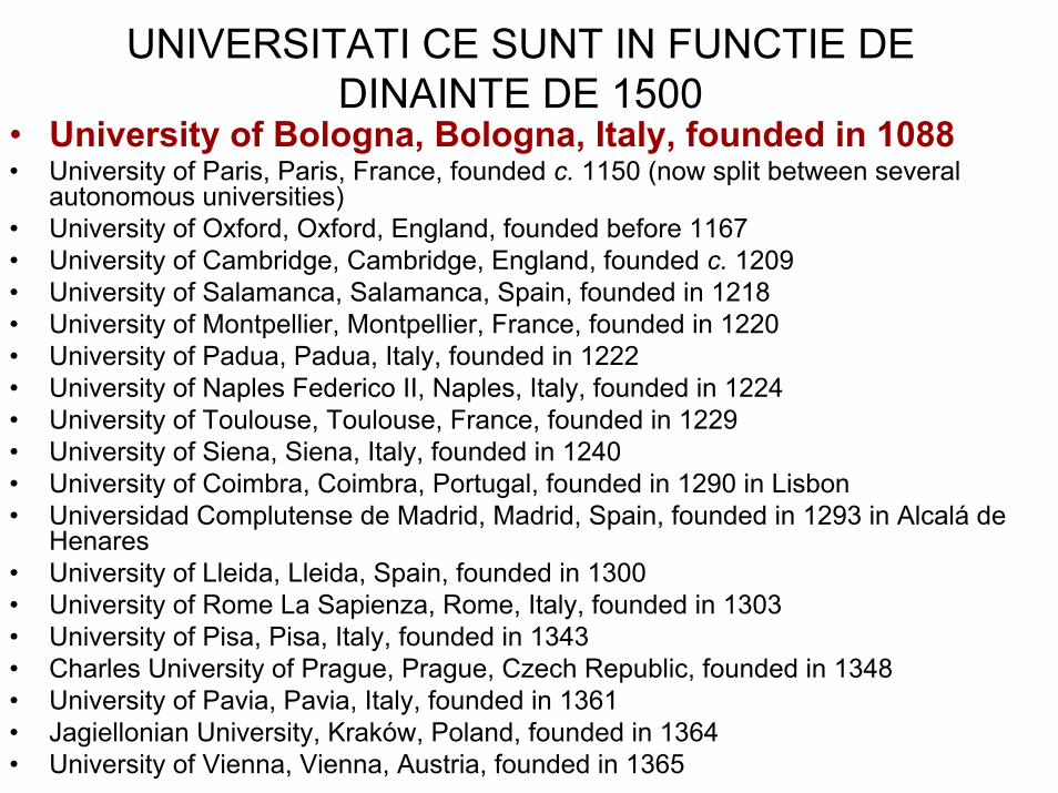
UNIVERSITATI CE SUNT IN FUNCTIE DE DINAINTE DE 1500

• University of Bologna, Bologna, Italy, founded in 1088• University of Paris, Paris, France, founded c. 1150 (now split between several

autonomous universities) • University of Oxford, Oxford, England, founded before 1167 • University of Cambridge, Cambridge, England, founded c. 1209 • University of Salamanca, Salamanca, Spain, founded in 1218 • University of Montpellier, Montpellier, France, founded in 1220 • University of Padua, Padua, Italy, founded in 1222 • University of Naples Federico II, Naples, Italy, founded in 1224• University of Toulouse, Toulouse, France, founded in 1229 • University of Siena, Siena, Italy, founded in 1240 • University of Coimbra, Coimbra, Portugal, founded in 1290 in Lisbon • Universidad Complutense de Madrid, Madrid, Spain, founded in 1293 in Alcalá de

Henares• University of Lleida, Lleida, Spain, founded in 1300 • University of Rome La Sapienza, Rome, Italy, founded in 1303 • University of Pisa, Pisa, Italy, founded in 1343 • Charles University of Prague, Prague, Czech Republic, founded in 1348 • University of Pavia, Pavia, Italy, founded in 1361 • Jagiellonian University, Kraków, Poland, founded in 1364 • University of Vienna, Vienna, Austria, founded in 1365

UNIVERSITATI CE SUNT IN FUNCTIE DE DINAINTE DE 1500

• University of Ferrara, Ferrara, Italy, founded in 1391 • University of Würzburg, Würzburg, Germany, founded in 1402 • University of Leipzig, Leipzig, Germany, founded in 1409 • University of St. Andrews, St. Andrews, Scotland, founded in 1412 • University of Rostock, Rostock, Germany, 1367 • Ruprecht Karls University of Heidelberg, Heidelberg founded in 1419 • Catholic University of Leuven, Leuven, Belgium, founded in 1425, now split between

the French-speaking Université catholique de Louvain, Louvain-la-Neuve and the Dutch-speaking Katholieke Universiteit Leuven, still at Leuven

• University of Poitiers, Poitiers, France, founded in 1431 • University of Pécs, Pécs, Hungary, founded in, Germany, founded in 1386 • University of Glasgow, Glasgow, Scotland, founded in 1451 • University of Istanbul, Istanbul, Turkey, founded in 1453 • Ernst Moritz Arndt University of Greifswald, Greifswald, Germany, founded in 1456 • Albert Ludwigs University of Freiburg, Freiburg, Germany, founded in 1457 • Basel University, Basel, Switzerland, founded in 1460 • Uppsala University, Uppsala, Sweden, founded in 1477 • Eberhard Karls University of Tübingen, Tübingen, Germany, founded in 1477 • University of Copenhagen, Copenhagen, Denmark, founded in 1479 • University of Aberdeen, Aberdeen, Scotland, founded in 1494 • University of Santiago de Compostela, Galicia, Spain, founded in 1495

UNIVERSITATEA DIN BOLOGNA A FOST INTOTDEAUNA UNA DE AVANGARDA

Laura Maria Caterina Bassi (1711 –1778)

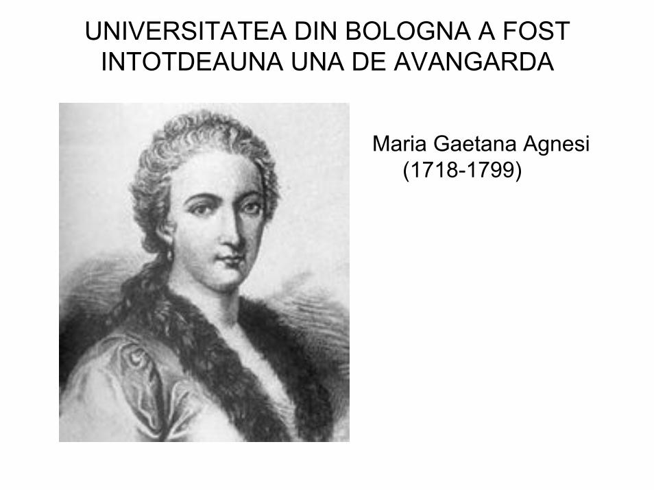
UNIVERSITATEA DIN BOLOGNA A FOST INTOTDEAUNA UNA DE AVANGARDA

Maria Gaetana Agnesi(1718-1799)

PROBABIL DIN REGIUNEA LUI VA VENI URMATOAREA SCHIMBARE

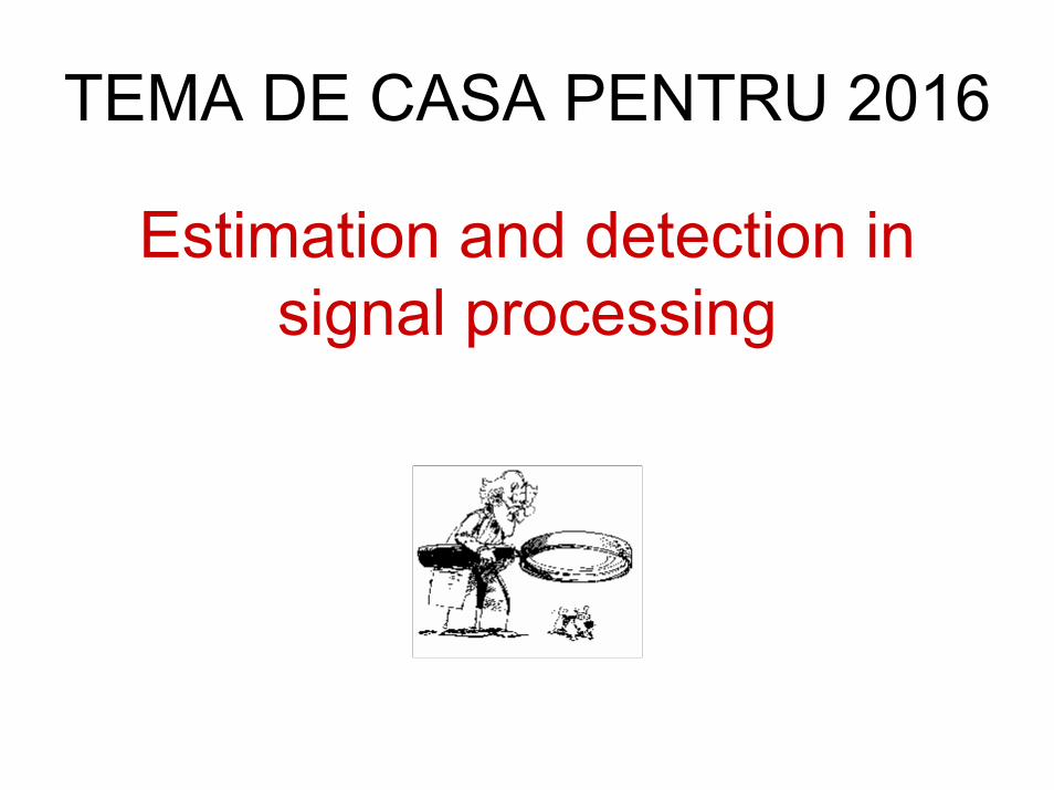
TEMA DE CASA PENTRU 2016

Estimation and detection in signal processing

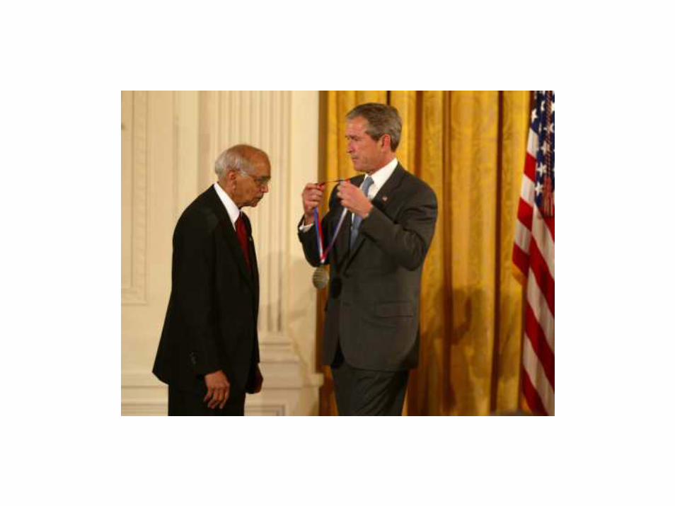
Professor C.R. Rao received National Medal of Science "for his pioneering contributions to the foundations of statistical theory and multivariate statistical methodology and their applications, enriching the physical, biological, mathematical, economic and engineering sciences."

Estimation in signal processingModern estimation theory can be found at the heart of many electronic signal processing systems, designed to extract information:

• Radar• Sonar• Speech analysis• Image analysis

– e.g. estimate the position and orientation of an object from a camera image in robotics

• Biomedicine – e.g. estimate the heart rate of a fetus

• Communications – e.g. estimate the carrier frequency of a signal so that the signal can be

demodulated to baseband• Control• Seismology

– estimate the underground distance of an oil deposit based on the sound reflections

and all share the common problem of needing to estimate the value of a group of parameters.

Estimation in signal processing (cont’d)

a) Radar b) Transmit & received waveforms

Fig. 1: Radar system

02 (1)Rc

τ =

Estimation in signal processing (cont’d)

Fig.2b Received signals at array sensors

Fig.2a: Passive sonar

Fig. 2: Passive sonar system

0arccos (2)cdτβ ⎛ ⎞= ⎜ ⎟

⎝ ⎠

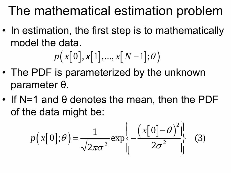
The mathematical estimation problem• In estimation, the first step is to mathematically

model the data.

• The PDF is parameterized by the unknown parameter θ.

• If N=1 and θ denotes the mean, then the PDF of the data might be:

[ ] [ ] [ ]( )0 , 1 ,..., 1 ;p x x x N θ−

[ ]( ) [ ]( )2

22

010 ; exp (3)22

xp x

θθ

σπσ

⎧ ⎫−⎪ ⎪= −⎨ ⎬⎪ ⎪⎩ ⎭

The mathematical estimation problem (cont’d)

Fig.3 Dependence of PDF on unknown parameter

Fig.4 Hypothetical Dow-Jones average

The mathematical estimation problem (cont’d)

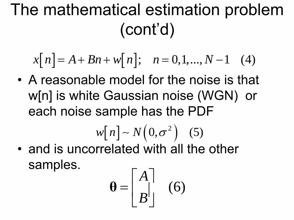
• A reasonable model for the noise is that w[n] is white Gaussian noise (WGN) or each noise sample has the PDF

• and is uncorrelated with all the other samples.

[ ] [ ]; 0,1,..., 1 (4)x n A Bn w n n N= + + = −

[ ] ( )20, (5)w n N σ∼

(6)AB⎡ ⎤

= ⎢ ⎥⎣ ⎦

θ

The mathematical estimation problem (cont’d)

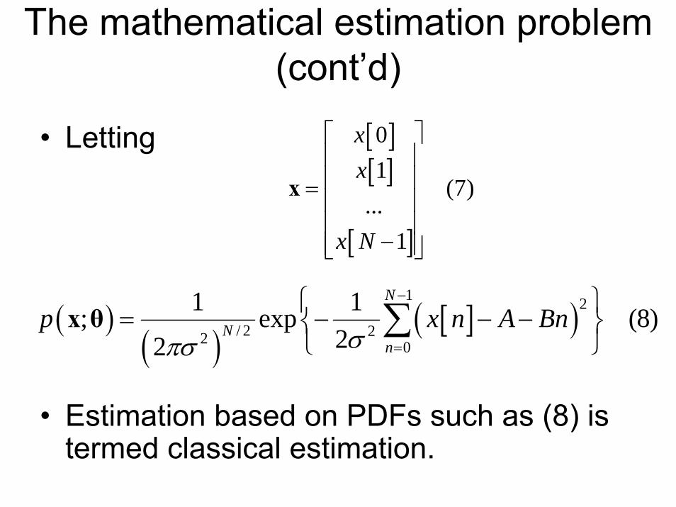
• Letting

• Estimation based on PDFs such as (8) is termed classical estimation.

[ ][ ]

[ ]

01

(7)...

1

xx

x N

⎡ ⎤⎢ ⎥⎢ ⎥= ⎢ ⎥⎢ ⎥

−⎢ ⎥⎣ ⎦

x

( )( )

[ ]( )1 2

/ 2 22 0

1 1; exp (8)22

N

Nn

p x n A Bnσπσ

−

=

⎧ ⎫= − − −⎨ ⎬

⎩ ⎭∑x θ

The Bayesian estimation

• The parameter we are attempting to estimate is then viewed as a realization of the random variable θ. As such, the data is described by the joint PDF:

( ) ( ) ( ), (9)p p pθ θ θ=x x

[ ] [ ] [ ]( ) ( )ˆ 0 , 1 ,..., 1 (10)g x x x N gθ = − = x

The Bayesian estimation (cont’d)

• An estimator is a rule that assigns a value to θ for each realization of x.

• The estimate of θ is the value of θobtained for a given realization of x. This distinction is analogous to a random variable (a function defined on the sample space) and the value it takes on.

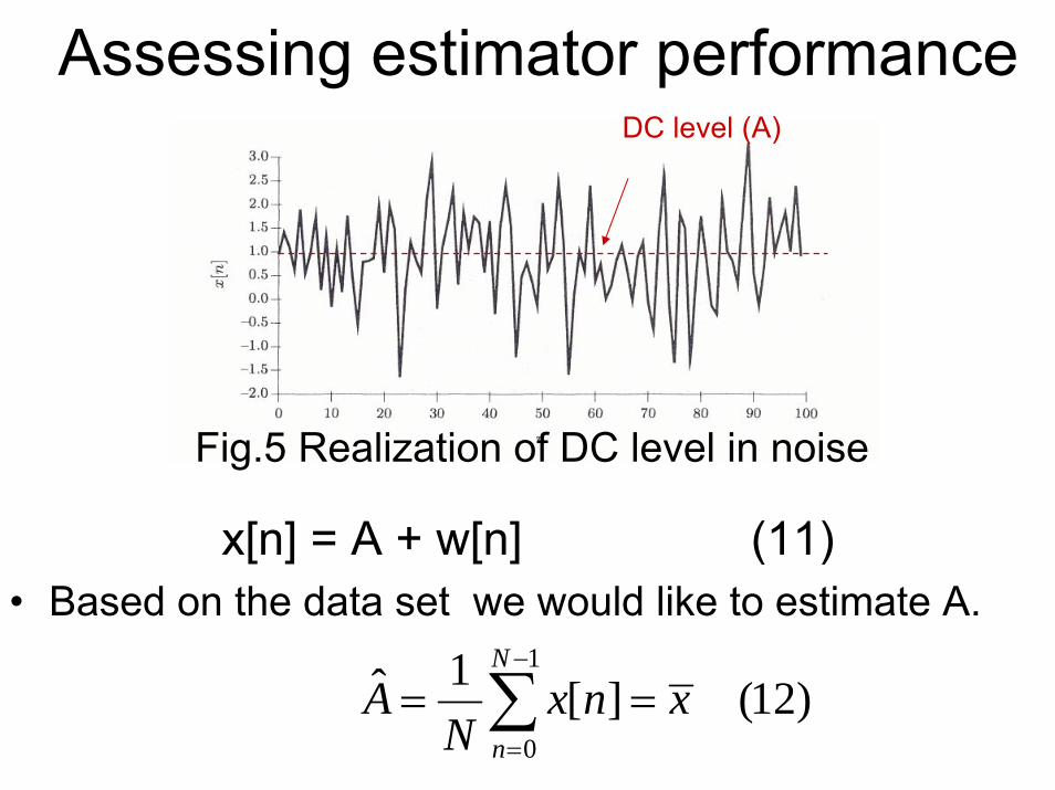
Assessing estimator performance

x[n] = A + w[n] (11) • Based on the data set we would like to estimate A.

1

0

1ˆ [ ] (12)N

nA x n x

N

−

=

= =∑

Fig.5 Realization of DC level in noise

DC level (A)

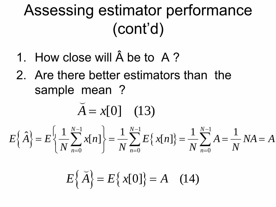
Assessing estimator performance (cont’d)

1. How close will  be to A ?2. Are there better estimators than the

sample mean ?

[0] (13)A x=

{ } { }1 1 1

0 0 0

1 1 1 1ˆ [ ] [ ]N N N

n n nE A E x n E x n A NA A

N N N N

− − −

= = =

⎧ ⎫= = = = =⎨ ⎬

⎩ ⎭∑ ∑ ∑

{ } { }[0] (14)E A E x A= =

Assessing estimator performance (cont’d)

{ } { }21 1 1

22 2

0 0 0

1 1 1ˆvar var [ ] var [ ]N N N

n n nA x n x n

N N N Nσσ

− − −

= = =

⎧ ⎫= = = =⎨ ⎬

⎩ ⎭∑ ∑ ∑

{ } { } { } { }2 ˆvar var [0] var var (15)A x A Aσ= = >

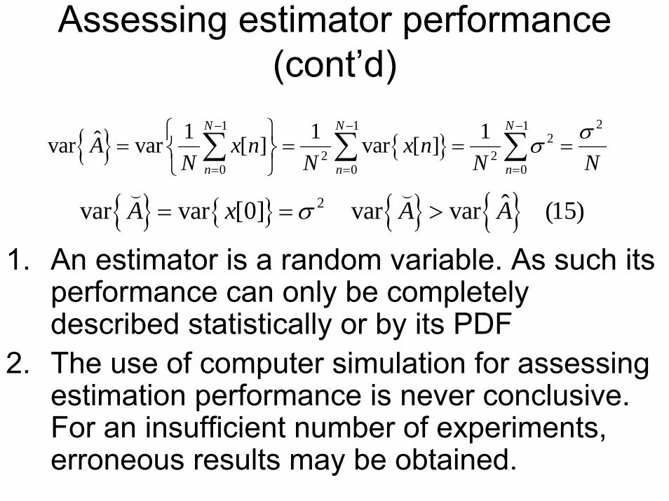
1. An estimator is a random variable. As such its performance can only be completely described statistically or by its PDF

2. The use of computer simulation for assessing estimation performance is never conclusive. For an insufficient number of experiments, erroneous results may be obtained.

Minimum variance unbiased estimators

Unbiased estimators• Mathematically, an estimator is unbiased if

• Multiple estimates of the same parameter are available, i.e.

{ }ˆ (16)E θ θ θ= ∀

{ }1 2ˆ ˆ ˆ, ,..., nθ θ θ

1

1ˆ ˆ (17)n

iin

θ θ=

= ∑

MVU estimators (cont’d)

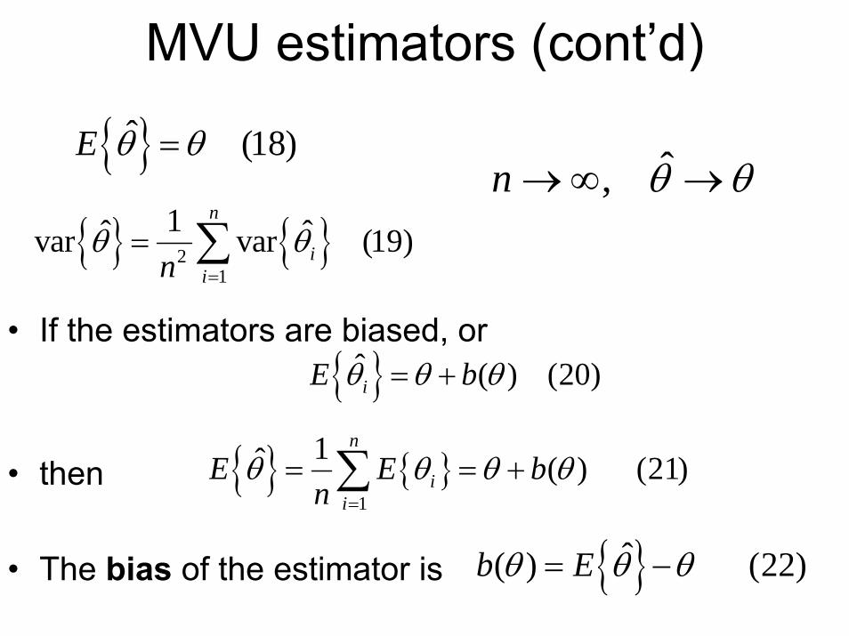
{ }ˆ (18)E θ θ= ˆ,n θ θ→ ∞ →

{ } { }21

1ˆ ˆvar var (19)n

iin

θ θ=

= ∑

• If the estimators are biased, or

• then

• The bias of the estimator is

{ }ˆ ( ) (20)iE bθ θ θ= +

{ } { }1

1ˆ ( ) (21)n

ii

E E bn

θ θ θ θ=

= = +∑

{ }ˆ( ) (22)b Eθ θ θ= −

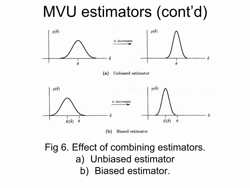
MVU estimators (cont’d)

Fig 6. Effect of combining estimators.a) Unbiased estimator b) Biased estimator.

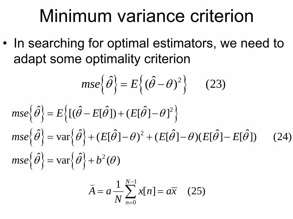
Minimum variance criterion• In searching for optimal estimators, we need to

adapt some optimality criterion

{ } { }2ˆ ˆ( ) (23)mse Eθ θ θ= −

{ } { }{ } { }{ } { }

2

2

2

ˆ ˆ ˆ ˆ[( [ ]) ( [ ] ]

ˆ ˆ ˆ ˆ ˆ ˆvar ( [ ] ) ( [ ] )( [ ] [ ]) (24)

ˆ ˆvar ( )

mse E E E

mse E E E E

mse b

θ θ θ θ θ

θ θ θ θ θ θ θ θ

θ θ θ

= − + −

= + − + − −

= +

1

0

1 [ ] (25)N

nA a x n ax

N

−

=

= =∑

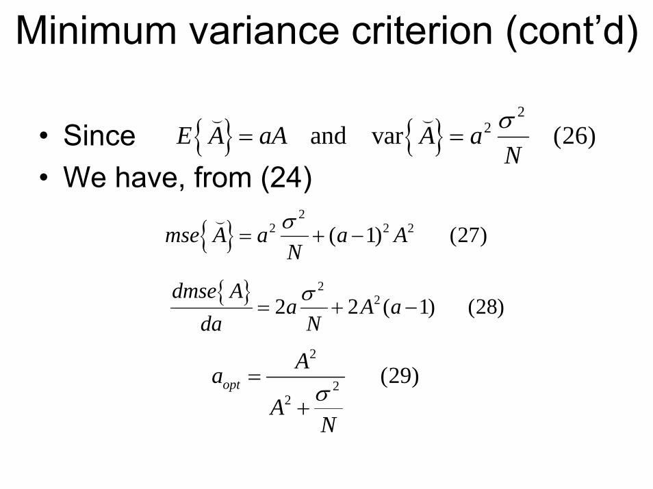
Minimum variance criterion (cont’d)

• Since• We have, from (24)

{ } { }2

2and var (26)E A aA A aNσ

= =

{ }2

2 2 2( 1) (27)mse A a a ANσ

= + −

{ } 222 2 ( 1) (28)

dmse Aa A a

da Nσ

= + −

2

22

(29)optAa

ANσ

=+

Minimum variance criterion (cont’d)

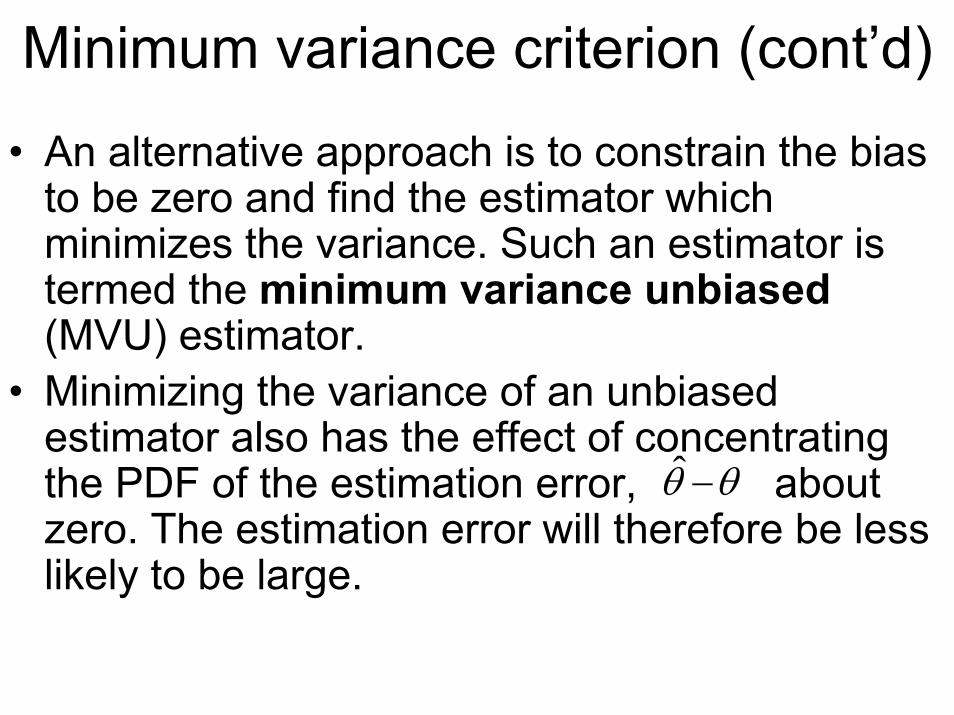
• An alternative approach is to constrain the bias to be zero and find the estimator which minimizes the variance. Such an estimator is termed the minimum variance unbiased(MVU) estimator.

• Minimizing the variance of an unbiased estimator also has the effect of concentrating the PDF of the estimation error, about zero. The estimation error will therefore be less likely to be large.

θ̂ θ−

Existence of the MVU estimator

a) is the MVU estimator

Fig.7: Possible dependence of the estimator variance with θ.

3̂θ b) There is no MVU estimator

Finding the MVU estimator

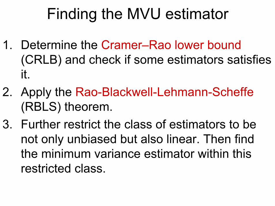
1. Determine the Cramer–Rao lower bound(CRLB) and check if some estimators satisfies it.

2. Apply the Rao-Blackwell-Lehmann-Scheffe(RBLS) theorem.

3. Further restrict the class of estimators to be not only unbiased but also linear. Then find the minimum variance estimator within this restricted class.

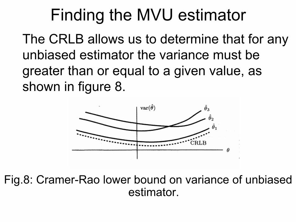
Finding the MVU estimator The CRLB allows us to determine that for any unbiased estimator the variance must be greater than or equal to a given value, as shown in figure 8.

Fig.8: Cramer-Rao lower bound on variance of unbiased estimator.

Estimator accuracy consideration • Since all our information is embodied in the

observed data and the underlying PDF for the data, the estimation accuracy depend directly on the PDF.

• If a single sample is observed as

• A good unbiased estimator is:Â = x[0] (31)

( )2[0] [0]; [0] 0, (30)x A w w N σ= + ∼

Estimator accuracy consideration (cont’d)

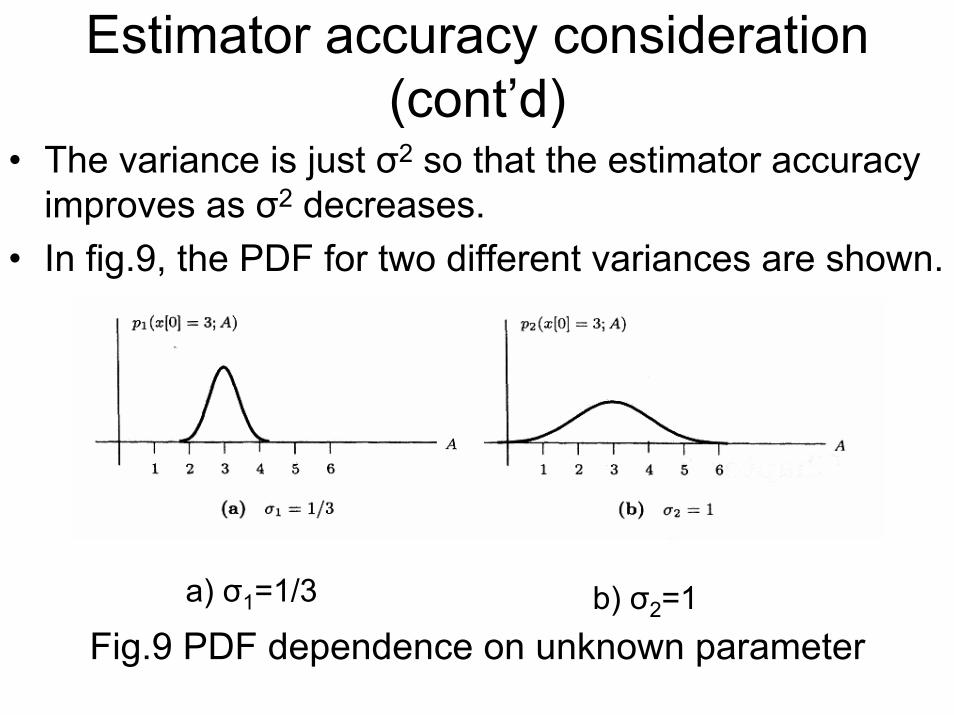
• The variance is just σ2 so that the estimator accuracy improves as σ2 decreases.

• In fig.9, the PDF for two different variances are shown.

a) σ1=1/3 b) σ2=1Fig.9 PDF dependence on unknown parameter

Estimator accuracy consideration (cont’d)

222

1 1( [0]; ) exp ( [0] ) ; 1,2 (32)22

iii

p x A x A iσπσ

⎧ ⎫= − − =⎨ ⎬

⎩ ⎭

• If x[0]=3 and σ1=1/3 values of A in the interval [3-3σ1,3+3σ1]=[2,4] are viable candidates.

• When the PDF is viewed as a function of the unknown parameter (x fixed), it is termed the “likelihood function”.

• The “sharpness” of the likelihood function determines how accurately we can estimates the unknown parameter.

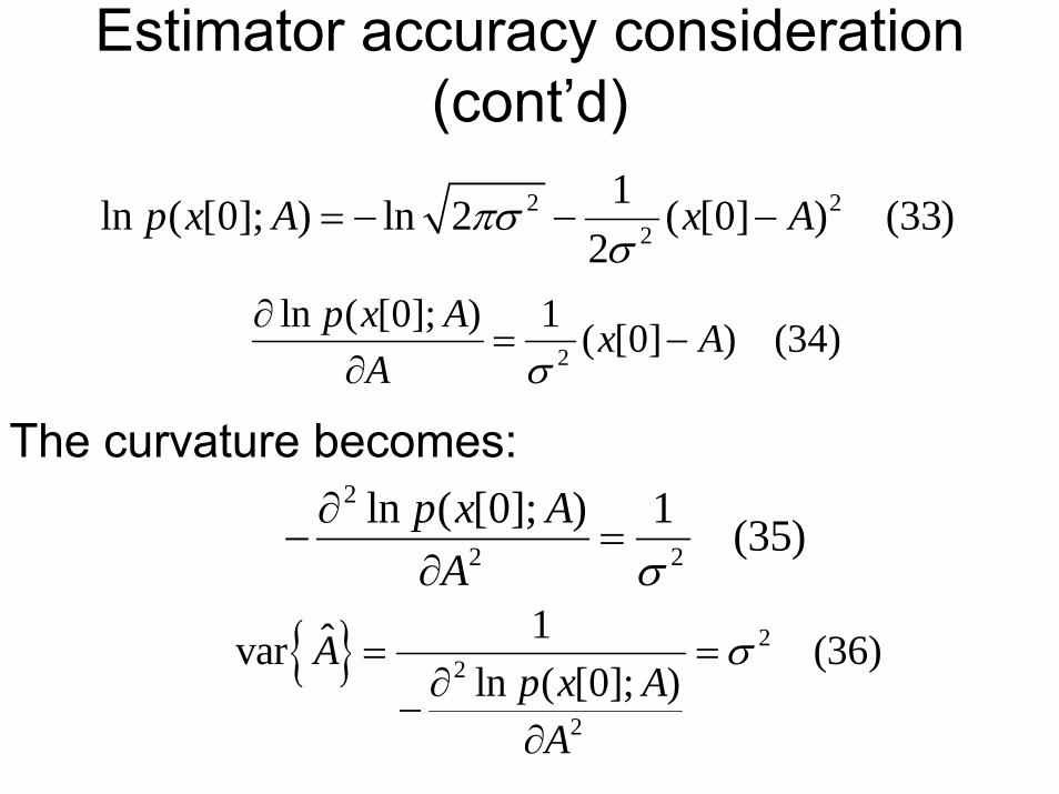
Estimator accuracy consideration (cont’d)

2 22

1ln ( [0]; ) ln 2 ( [0] ) (33)2

p x A x Aπσσ

= − − −

2

ln ( [0]; ) 1 ( [0] ) (34)p x A x AA σ

∂= −

∂

The curvature becomes:2

2 2

ln ( [0]; ) 1 (35)p x AA σ

∂− =

∂

{ } 22

2

1ˆvar (36)ln ( [0]; )

Ap x A

A

σ= =∂

−∂

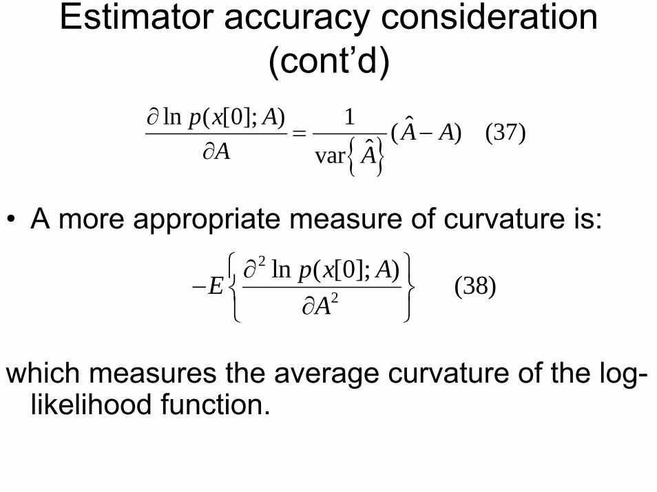
Estimator accuracy consideration (cont’d)

{ }ln ( [0]; ) 1 ˆ( ) (37)

ˆvarp x A A A

A A∂

= −∂

• A more appropriate measure of curvature is:

which measures the average curvature of the log-likelihood function.

2

2

ln ( [0]; ) (38)p x AEA

⎧ ⎫∂− ⎨ ⎬∂⎩ ⎭

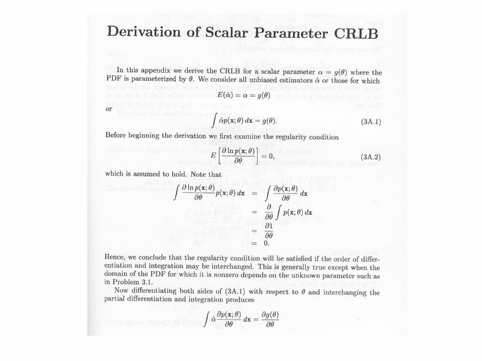
Theorem 1: Cramer-Rao Lower Bound, Scalar parameter

• It is assumed that the PDF, p(x; θ) satisfies the “regularity” condition:

where the expectation is taken with respect to p(x; θ).

ln ( ; ) 0, (39)pE θ θθ

∂⎧ ⎫ = ∀⎨ ⎬∂⎩ ⎭

x

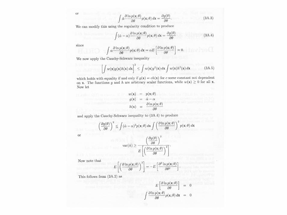
Theorem 1: Cramer-Rao Lower Bound, Scalar parameter (cont’d)

• Then, the variance of any unbiased estimator θmust satisfy

where the derivative is evaluated at the true value of θ and the expectation is taken with the respect to p(x;θ).

{ } 2

2

1ˆvar (40)ln ( ; )pE

θθ

θ

≥⎧ ⎫∂

− ⎨ ⎬∂⎩ ⎭

x

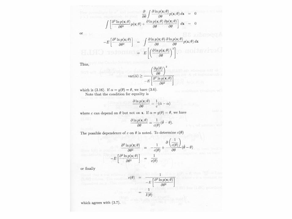
Theorem 1: Cramer-Rao Lower Bound, Scalar parameter (cont’d)

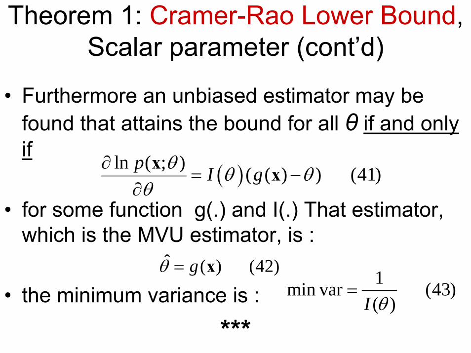
• Furthermore an unbiased estimator may be found that attains the bound for all θ if and only if

• for some function g(.) and I(.) That estimator, which is the MVU estimator, is :

• the minimum variance is :

***

( )ln ( ; ) ( ( ) ) (41)p I gθ θ θθ

∂= −

∂x x

ˆ ( ) (42)gθ = x 1min var (43)( )I θ

=

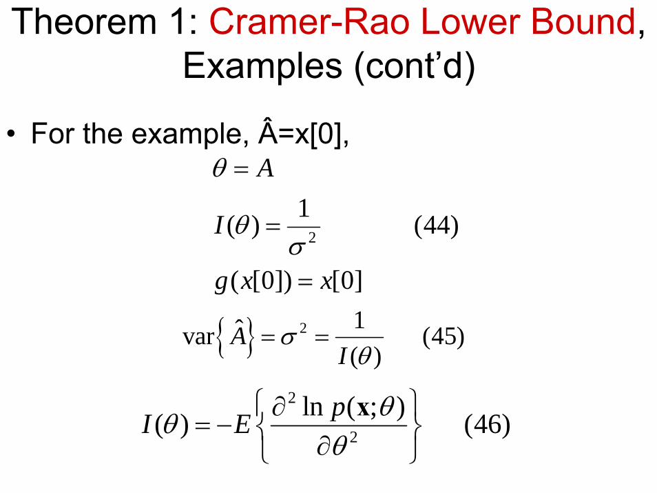
Theorem 1: Cramer-Rao Lower Bound, Examples (cont’d)

• For the example, Â=x[0],

2

1( ) (44)

( [0]) [0]

A

I

g x x

θ

θσ

=

=

=

{ } 2 1ˆvar (45)( )

AI

σθ

= =

2

2

ln ( ; )( ) (46)pI E θθθ

⎧ ⎫∂= − ⎨ ⎬∂⎩ ⎭

x

Theorem 1: Cramer-Rao Lower Bound, Examples (cont’d)

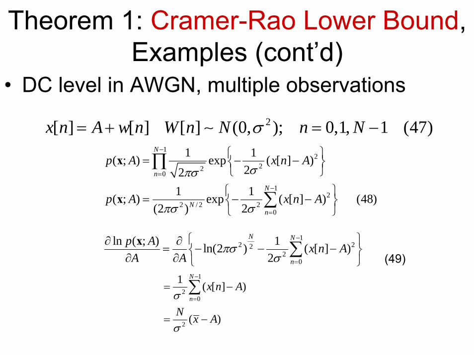
• DC level in AWGN, multiple observations 2[ ] [ ] [ ] (0, ); 0,1, 1 (47)x n A w n W n N n Nσ= + = −∼

12

220

12

2 / 2 20

1 1( ; ) exp ( [ ] )22

1 1( ; ) exp ( [ ] ) (48)(2 ) 2

N

n

N

Nn

p A x n A

p A x n A

σπσ

πσ σ

−

=

−

=

⎧ ⎫= − −⎨ ⎬⎩ ⎭

⎧ ⎫= − −⎨ ⎬

⎩ ⎭

∏

∑

x

x

12 22

20

ln ( ; ) 1ln(2 ) ( [ ] )2

N N

n

p A x n AA A

πσσ

−

=

⎧ ⎫∂ ∂= − − −⎨ ⎬∂ ∂ ⎩ ⎭

∑x

1

20

2

1 ( [ ] )

( )

N

nx n A

N x A

σ

σ

−

=

= −

= −

∑

(49)

Theorem 1: Cramer-Rao Lower Bound, Examples (cont’d)

{ }

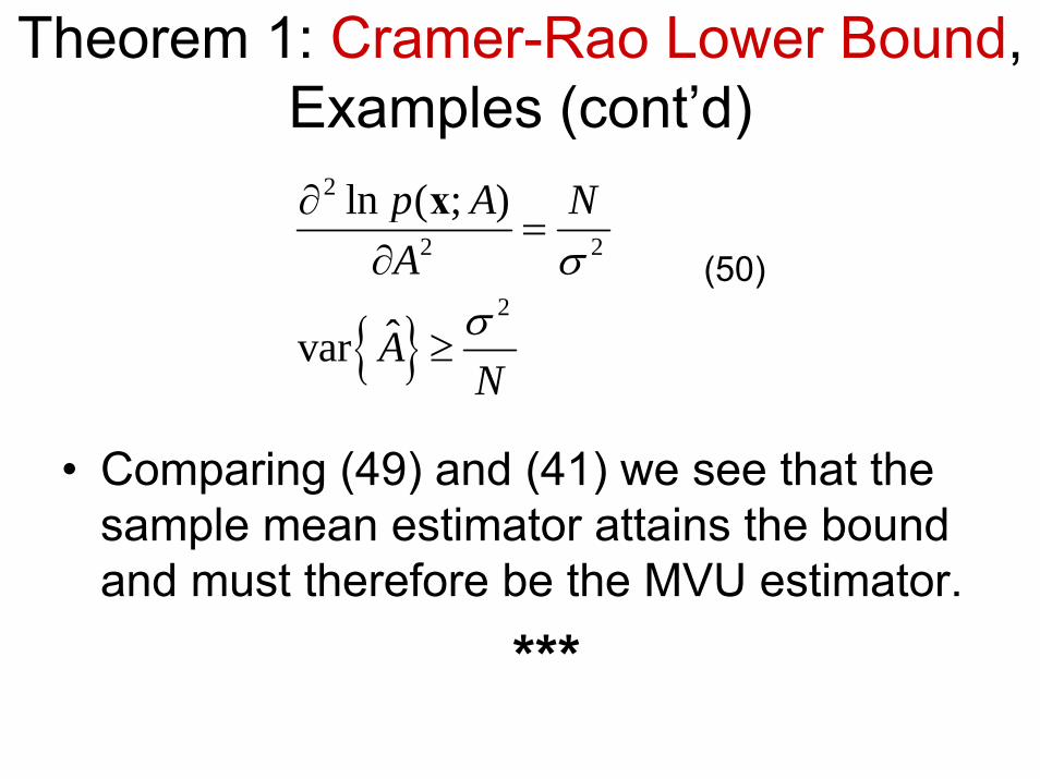
2

2 2

2

ln ( ; )

ˆvar

p A NA

AN

σσ

∂=

∂

≥

x(50)

• Comparing (49) and (41) we see that the sample mean estimator attains the bound and must therefore be the MVU estimator.

***

• We prove that when CRLB is attained

• From (41) and (42)

{ } 1ˆvar (51)( )I

θθ

=

2

2

ln ( ; )( ) (52)pI E θθθ

⎧ ⎫∂= − ⎨ ⎬∂⎩ ⎭

x

{ } 2

2

1ˆvar (53)ln ( ; )pE

θθ

θ

=⎧ ⎫∂

− ⎨ ⎬∂⎩ ⎭

x

ln ( ; ) ˆ( )( ) (54)p Iθ θ θ θθ

∂= −

∂x

Theorem 1: Cramer-Rao Lower Bound, Examples (cont’d)

Theorem 1: Cramer-Rao Lower Bound, Examples (cont’d)

2

2

ln ( ; ) ( ) ˆ( ) ( ) (55)p I Iθ θ θ θ θθ θ

∂ ∂= − −

∂ ∂x

{ }2

2

ln ( ; ) ( ) ˆ( ) ( ) ( ) (56)p IE E I Iθ θ θ θ θ θθ θ

⎧ ⎫∂ ∂− = − − + =⎨ ⎬∂ ∂⎩ ⎭

x

• And therefore

{ } 1ˆvar( )I

θθ

=

Theorem 1: Cramer-Rao Lower Bound, Examples (cont’d)

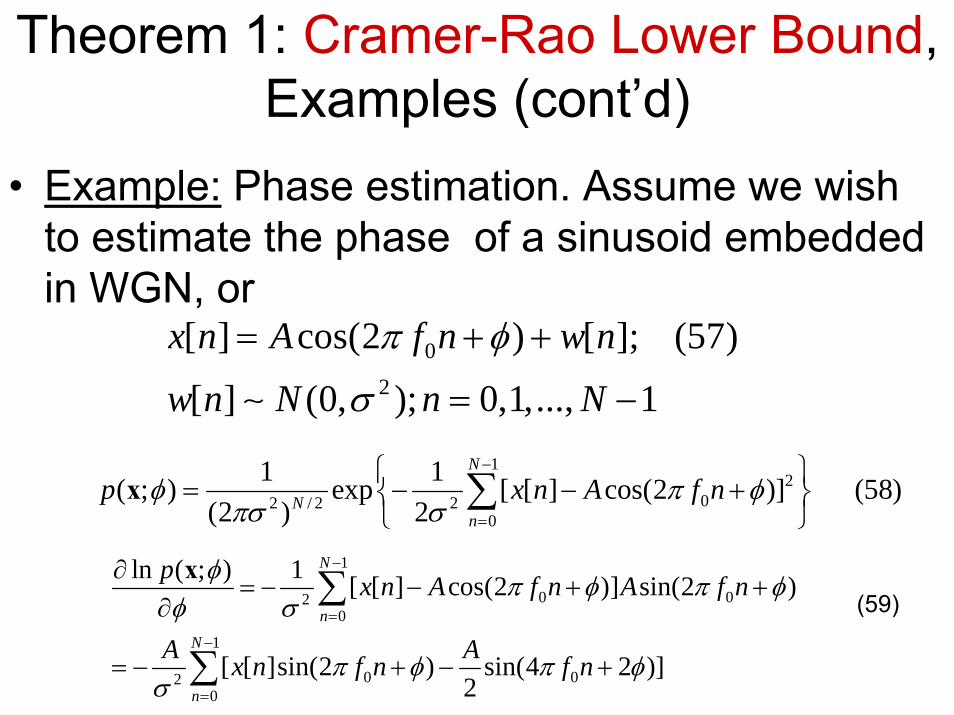
• Example: Phase estimation. Assume we wish to estimate the phase of a sinusoid embedded in WGN, or

02

[ ] cos(2 ) [ ]; (57)

[ ] (0, ); 0,1,..., 1

x n A f n w nw n N n N

π φ

σ

= + +

= −∼1

202 / 2 2

0

1 1( ; ) exp [ [ ] cos(2 )] (58)(2 ) 2

N

Nn

p x n A f nφ π φπσ σ

−

=

⎧ ⎫= − − +⎨ ⎬

⎩ ⎭∑x

1

0 020

1

0 020

ln ( ; ) 1 [ [ ] cos(2 )] sin(2 )

[ [ ]sin(2 ) sin(4 2 )]2

N

n

N

n

p x n A f n A f n

A Ax n f n f n

φ π φ π φφ σ

π φ π φσ

−

=

−

=

∂= − − + +

∂

= − + − +

∑

∑

x(59)

Theorem 1: Cramer-Rao Lower Bound, Examples (cont’d)

[ ]2 1

0 02 20

ln ( ; ) [ ]cos(2 ) cos(4 2 ) (60)N

n

p A x n f n A f nφ π φ π φφ σ

−

=

∂= − + − +

∂ ∑x

{ }2 1

0 02 20

12

0 0201

0 020

2

2

ln ( ; ) [ [ ] cos(2 ) cos(4 2 )]

[ cos (2 ) cos(4 2 )]

1 1[ cos(4 2 ) cos(4 2 )]2 2

2

N

n

N

nN

n

p AE E x n f n A f n

A A f n A f n

A f n A f n

NA

θ π φ π φθ σ

π φ π φσ

π φ π φσ

σ

−

=

−

=

−

=

⎧ ⎫∂− = + − + =⎨ ⎬∂⎩ ⎭

= + − +

= + + − +

≅

∑

∑

∑

x

(61)

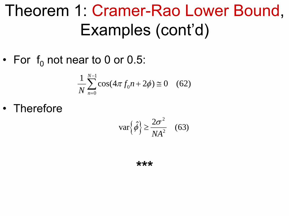
Theorem 1: Cramer-Rao Lower Bound, Examples (cont’d)

• For f0 not near to 0 or 0.5:

• Therefore

***

1

00

1 cos(4 2 ) 0 (62)N

nf n

Nπ φ

−

=

+ ≅∑

{ }2

2

2ˆvar (63)NAσφ ≥

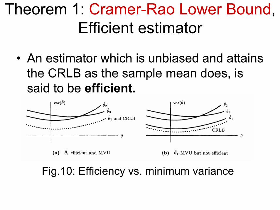
Theorem 1: Cramer-Rao Lower Bound, Efficient estimator

• An estimator which is unbiased and attains the CRLB as the sample mean does, is said to be efficient.

Fig.10: Efficiency vs. minimum variance

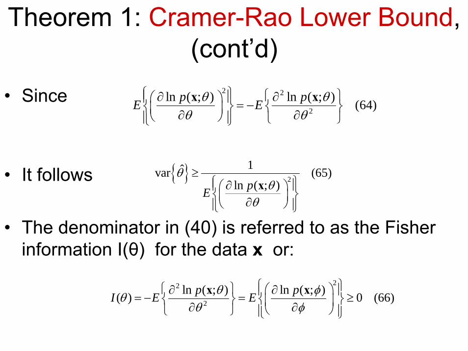
Theorem 1: Cramer-Rao Lower Bound, (cont’d)

• Since

• It follows

• The denominator in (40) is referred to as the Fisher information I(θ) for the data x or:

2 2

2

ln ( ; ) ln ( ; ) (64)p pE Eθ θθ θ

⎧ ⎫ ⎧ ⎫∂ ∂⎪ ⎪⎛ ⎞ = −⎨ ⎬ ⎨ ⎬⎜ ⎟∂ ∂⎝ ⎠ ⎩ ⎭⎪ ⎪⎩ ⎭

x x

22

2

ln ( ; ) ln ( ; )( ) 0 (66)p pI E Eθ φθθ φ

⎧ ⎫⎧ ⎫ ⎛ ⎞∂ ∂⎪ ⎪= − = ≥⎨ ⎬ ⎨ ⎬⎜ ⎟∂ ∂⎝ ⎠⎩ ⎭ ⎪ ⎪⎩ ⎭

x x

{ } 2

1ˆvar (65)ln ( ; )pE

θθ

θ

≥⎧ ⎫∂⎪ ⎪⎛ ⎞⎨ ⎬⎜ ⎟∂⎝ ⎠⎪ ⎪⎩ ⎭

x

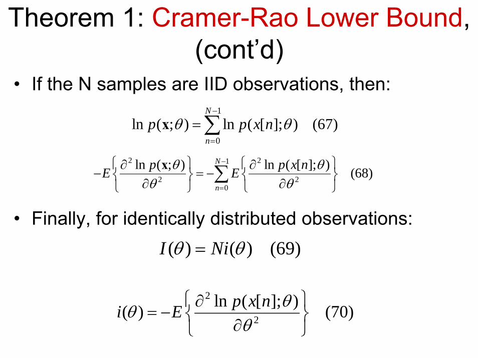
• If the N samples are IID observations, then:

• Finally, for identically distributed observations:( ) ( ) (69)I Niθ θ=

Theorem 1: Cramer-Rao Lower Bound, (cont’d)

1

0ln ( ; ) ln ( [ ]; ) (67)

N

np p x nθ θ

−

=

= ∑x

2 21

2 20

ln ( ; ) ln ( [ ]; ) (68)N

n

p p x nE Eθ θθ θ

−

=

⎧ ⎫ ⎧ ⎫∂ ∂− = −⎨ ⎬ ⎨ ⎬∂ ∂⎩ ⎭ ⎩ ⎭

∑x

2

2

ln ( [ ]; )( ) (70)p x ni E θθθ

⎧ ⎫∂= − ⎨ ⎬∂⎩ ⎭

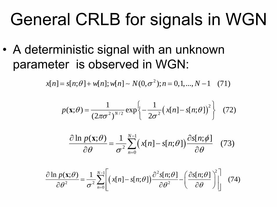
General CRLB for signals in WGN

• A deterministic signal with an unknown parameter is observed in WGN:

2[ ] [ ; ] [ ]; [ ] (0, ); 0,1,..., 1 (71)x n s n w n w n N n Nθ σ= + = −∼

( )22 / 2 2

1 1( ; ) exp [ ] [ ; ] (72)(2 ) 2Np x n s nθ θπσ σ

⎧ ⎫= − −⎨ ⎬⎩ ⎭

x

( )1

20

ln ( ; ) 1 [ ; ][ ] [ ; ] (73)N

n

p s nx n s nθ φθθ σ θ

−

=

∂ ∂= −

∂ ∂∑x

( )221

2 2 20

ln ( ; ) 1 [ ; ] [ ; ][ ] [ ; ] (74)N

n

p s n s nx n s nθ θ θθθ σ θ θ

−

=

⎡ ⎤∂ ∂ ∂⎛ ⎞= − −⎢ ⎥⎜ ⎟∂ ∂ ∂⎝ ⎠⎢ ⎥⎣ ⎦∑x

General CRLB for signals in WGN (cont’d){ }( )

221

2 2 20

21

20

ln ( ; ) 1 [ ; ] [ ; ][ ] [ ; ](75)

1 [ ; ]

N

n

N

n

p s n s nE E x n s n

s n

θ θ θθθ σ θ θ

θσ θ

−

=

−

=

⎡ ⎤∂ ∂ ∂⎧ ⎫ ⎛ ⎞= − −⎢ ⎥⎨ ⎬ ⎜ ⎟∂ ∂ ∂⎩ ⎭ ⎝ ⎠⎢ ⎥⎣ ⎦

∂⎛ ⎞= − ⎜ ⎟∂⎝ ⎠

∑

∑

x

{ }2

21

0

ˆvar (76)[ ; ]N

n

s nσθ

θθ

−

=

≥∂⎛ ⎞

⎜ ⎟∂⎝ ⎠∑

• Signals that change rapidly as the unknown parameter changes result in accurate estimators.

Example: Sinusoidal frequency estimation• We assume that the signal is sinusoidal and is

represented as

• From (76):

General CRLB for signals in WGN(cont’d)

( )0 0 0[ ; ] cos 2 ;0 1/ 2 (77)s n f A f n fπ φ= + ≤ <

{ }( )

2 2

0 21

00

/ˆvar (78)2 sin 2

N

n

Afn f n

σ

π π φ−

=

≥⎡ ⎤+⎣ ⎦∑

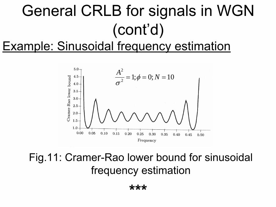
Example: Sinusoidal frequency estimation

***

General CRLB for signals in WGN(cont’d)

Fig.11: Cramer-Rao lower bound for sinusoidal frequency estimation

2

2 1; 0; 10A Nφσ

= = =

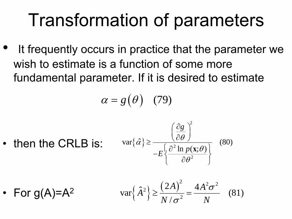
Transformation of parameters • It frequently occurs in practice that the parameter we

wish to estimate is a function of some more fundamental parameter. If it is desired to estimate

• then the CRLB is:

• For g(A)=A2

( ) (79)gα θ=

{ }

2

2

2

ˆvar (80)ln ( ; )

g

pE

θαθ

θ

∂⎛ ⎞⎜ ⎟∂⎝ ⎠≥

⎧ ⎫∂− ⎨ ⎬∂⎩ ⎭

x

{ } ( )2 2 22

2

2 4ˆvar (81)/A AA

N Nσ

σ≥ =

Transformation of parameters (cont’d)

• Since

• The efficiency is approximately maintained over nonlinear transformations if the data record is large enough.

2

, (82)x N ANσ⎛ ⎞

⎜ ⎟⎝ ⎠

∼

{ } { } { }22 2 2 2var (83)E x E x x A A

Nσ

= + = + ≠

{ } { } { }2 4 22var (84)x E x E x= −

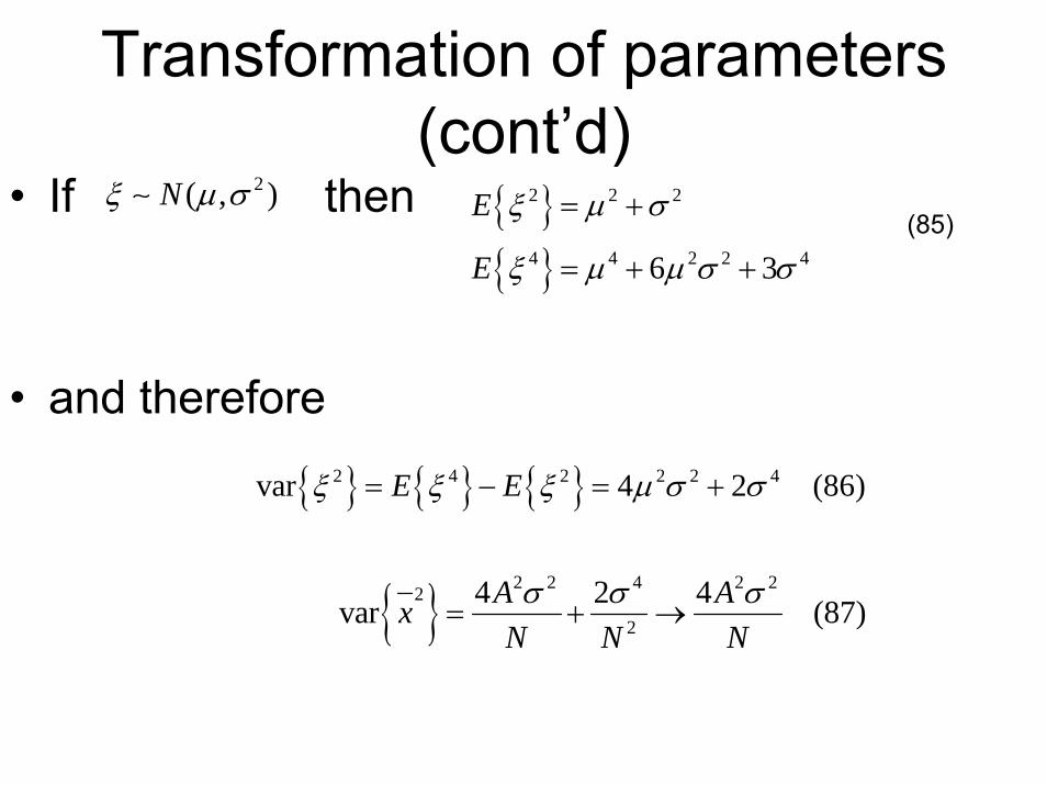
• If then

• and therefore

2( , )Nξ µ σ∼

Transformation of parameters (cont’d)

{ } { } { }2 4 2 2 2 4var 4 2 (86)E Eξ ξ ξ µ σ σ= − = +

{ }2 2 4 2 22

2

4 2 4var (87)A AxN N Nσ σ σ

= + →

{ }{ }

2 2 2

4 4 2 2 46 3

E

E

ξ µ σ

ξ µ µ σ σ

= +

= + +(85)

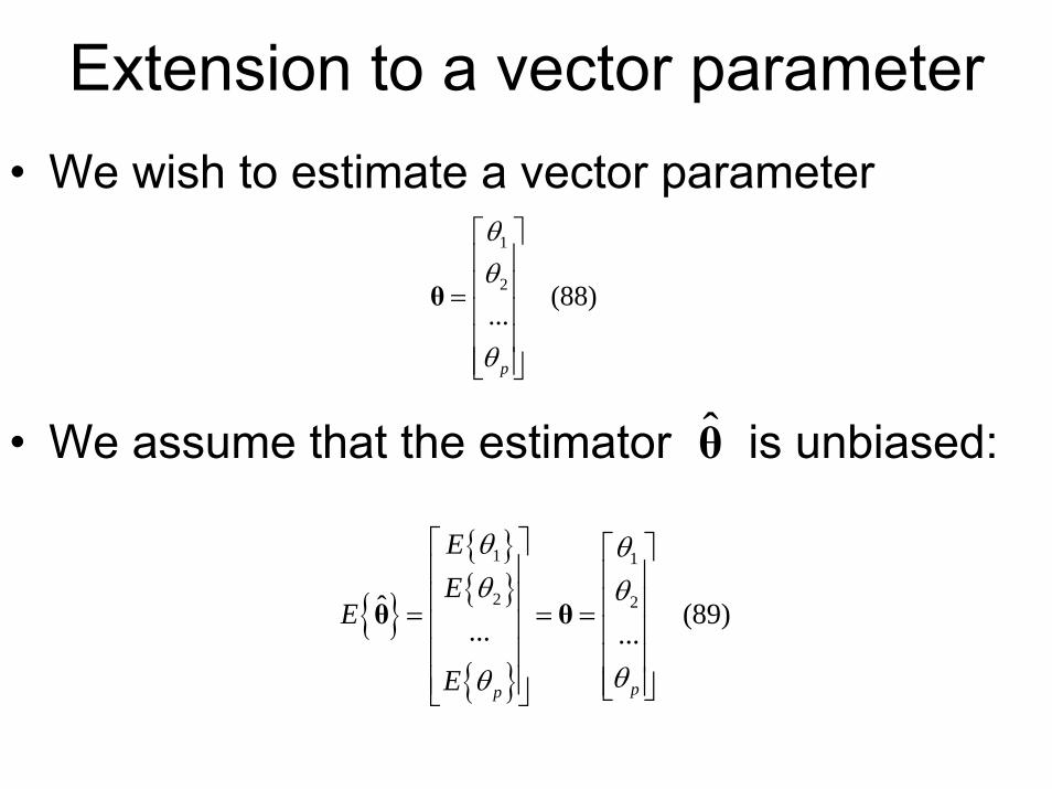
Extension to a vector parameter• We wish to estimate a vector parameter

• We assume that the estimator is unbiased:

1

2 (88)...

p

θθ

θ

⎡ ⎤⎢ ⎥⎢ ⎥=⎢ ⎥⎢ ⎥⎢ ⎥⎣ ⎦

θ

θ̂

{ }{ }{ }

{ }

1 1

2 2ˆ (89)... ...

pp

EE

E

E

θ θθ θ

θθ

⎡ ⎤ ⎡ ⎤⎢ ⎥ ⎢ ⎥⎢ ⎥ ⎢ ⎥= = =⎢ ⎥ ⎢ ⎥⎢ ⎥ ⎢ ⎥⎢ ⎥ ⎢ ⎥⎣ ⎦⎣ ⎦

θ θ

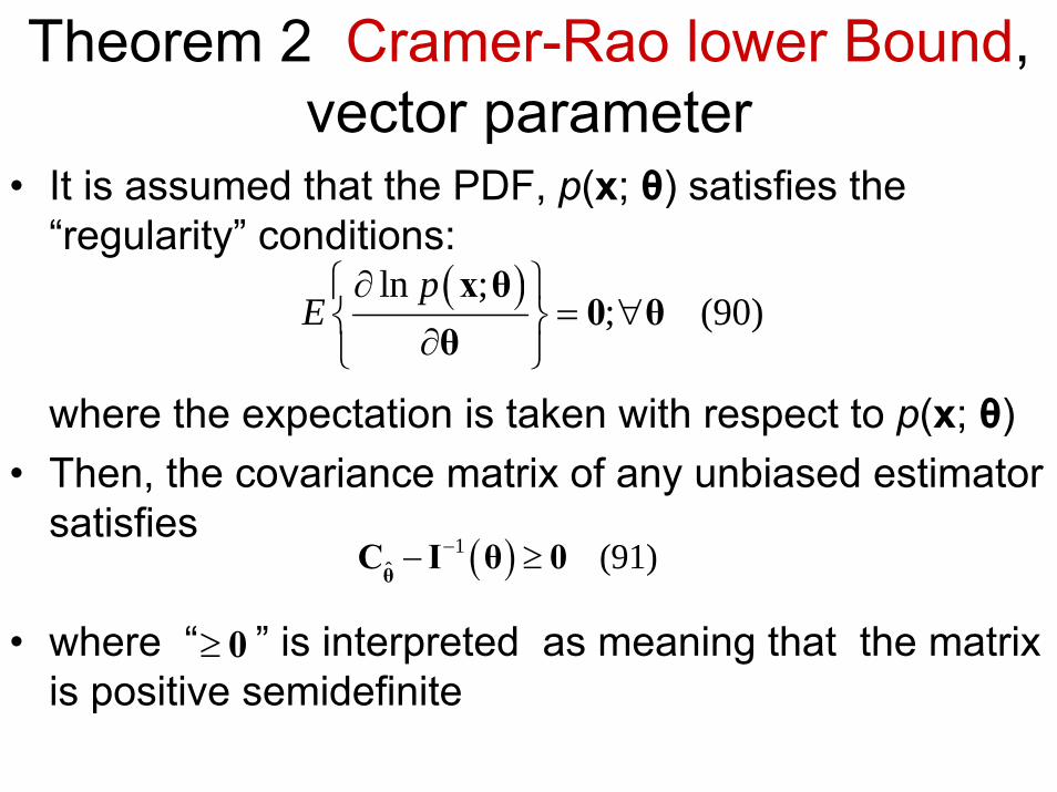
Theorem 2 Cramer-Rao lower Bound, vector parameter

• It is assumed that the PDF, p(x; θ) satisfies the “regularity” conditions:

where the expectation is taken with respect to p(x; θ) • Then, the covariance matrix of any unbiased estimator

satisfies

• where “ ” is interpreted as meaning that the matrix is positive semidefinite

( )ln ;; (90)

pE⎧ ⎫∂

= ∀⎨ ⎬∂⎩ ⎭

x θ0 θ

θ

( )1ˆ (91)−− ≥θC I θ 0

≥ 0

Theorem 2 Cramer-Rao lower Bound, vector parameter (cont’d)

• The Fisher information matrix I(θ) is given as:

where the derivatives are evaluated at the true value of θ and the expectation is taken with respect to p(x;θ).

• Furthermore, an unbiased estimator may be found that attains the bound in that

• if and only if

( ) ( )2 ln ;(92)

iji j

pE

θ θ⎧ ⎫∂⎪ ⎪⎡ ⎤ = − ⎨ ⎬⎣ ⎦ ∂ ∂⎪ ⎪⎩ ⎭

x θI θ

( )1ˆ (93)−=θC I θ

( ) ( ) ( )ln ;(94)

p∂⎡ ⎤= −⎣ ⎦∂

x θI θ g x θ

θ

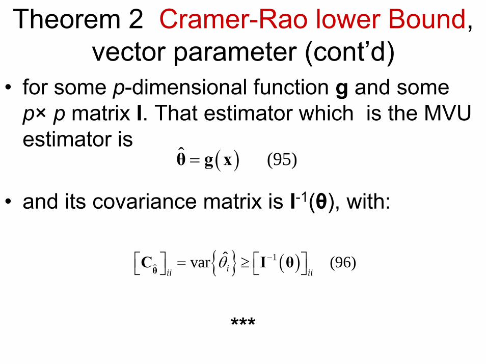
Theorem 2 Cramer-Rao lower Bound, vector parameter (cont’d)

• for some p-dimensional function g and some p× p matrix I. That estimator which is the MVU estimator is

• and its covariance matrix is I-1(θ), with:

***

( )ˆ (95)=θ g x

{ } ( )1ˆ

ˆvar (96)iii iiθ −⎡ ⎤ ⎡ ⎤= ≥⎣ ⎦ ⎣ ⎦θC I θ

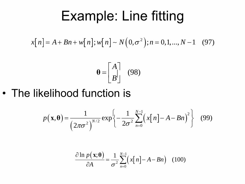
Example: Line fitting

• The likelihood function is

[ ] [ ] [ ] ( )2; 0, ; 0,1,..., 1 (97)x n A Bn w n w n N n Nσ= + + = −∼

(98)AB⎡ ⎤

= ⎢ ⎥⎣ ⎦

θ

( )( )

[ ]( )1 2

/ 2 22 0

1 1, exp (99)22

N

Nn

p x n A Bnσπσ

−

=

⎧ ⎫= − − −⎨ ⎬

⎩ ⎭∑x θ

( ) [ ]( )1

20

ln ; 1 (100)N

n

px n A Bn

A σ

−

=

∂= − −

∂ ∑x θ

Example: Line fitting (cont’d)

( ) [ ]( )1

20

ln ; 1 (101)N

n

px n A Bn n

B σ

−

=

∂= − −

∂ ∑x θ

( )2

2 2

ln ;(102)

p NA σ

∂= −

∂x θ

( ) ( )2 1

2 20

ln ; 11 1 (103)2

N

n

p N Nn

A B σ σ

−

=

∂ −= − = −

∂ ∂ ∑x θ

( ) ( )( )2 12

2 2 20

ln ; 1 2 11 1 (104)6

N

n

p N N Nn

B σ σ

−

=

∂ − −= − = −

∂ ∑x θ

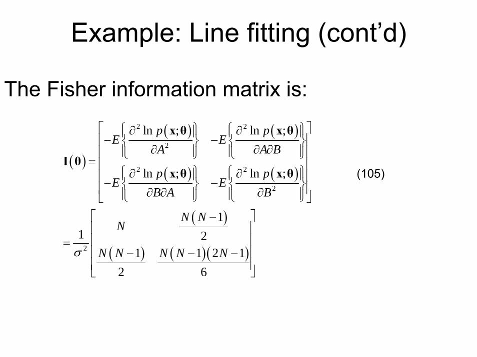
Example: Line fitting (cont’d)

The Fisher information matrix is:

( )

( ) ( )

( ) ( )

( )

( ) ( )( )

2 2

2

2 2

2

2

ln ; ln ;

ln ; ln ;

11 2

1 1 2 12 6

p pE E

A A B

p pE E

B A B

N NN

N N N N Nσ

⎡ ⎤⎧ ⎫ ⎧ ⎫∂ ∂⎪ ⎪ ⎪ ⎪− −⎢ ⎥⎨ ⎬ ⎨ ⎬∂ ∂ ∂⎪ ⎪ ⎪ ⎪⎢ ⎥⎩ ⎭ ⎩ ⎭= ⎢ ⎥⎧ ⎫ ⎧ ⎫∂ ∂⎪ ⎪ ⎪ ⎪⎢ ⎥− −⎨ ⎬ ⎨ ⎬⎢ ⎥∂ ∂ ∂⎪ ⎪ ⎪ ⎪⎩ ⎭ ⎩ ⎭⎣ ⎦

⎡ ⎤−⎢ ⎥⎢ ⎥=⎢ ⎥− − −⎢ ⎥⎣ ⎦

x θ x θ

I θx θ x θ (105)

Example: Line fitting (cont’d)

• It follows that:

( )

( )( ) ( )

( ) ( )

1 2

2

2 2 1 61 1

(106)6 12

1 1

NN N N N

N N N N

σ−

⎡ ⎤−−⎢ ⎥+ +⎢ ⎥= ⎢ ⎥

−⎢ ⎥+ −⎢ ⎥⎣ ⎦

I θ

{ } ( )( )

2 22 2 1 4ˆvar (107)1

NA

N N Nσ σ−

≥ →+

{ } ( )2 2

32

12 12ˆvar (108)1

BNN N

σ σ≥ →

−

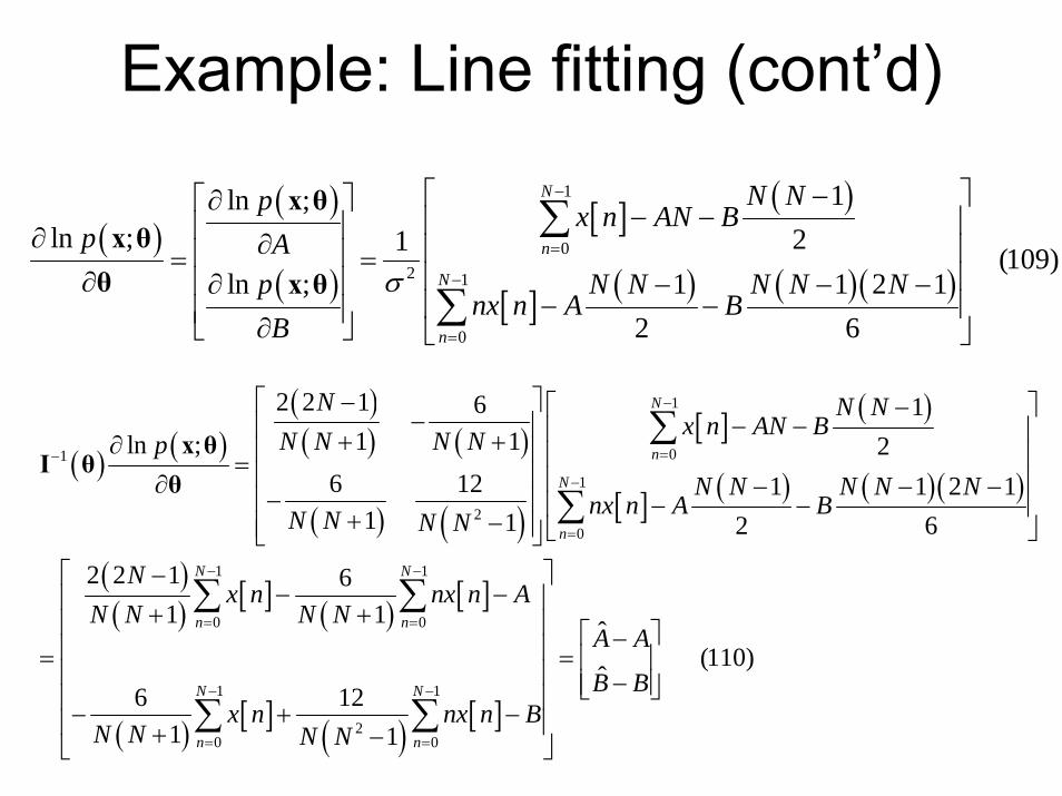
Example: Line fitting (cont’d)

( )( )

( )

[ ] ( )

[ ] ( ) ( )( )

1

02 1

0

1ln ;ln ; 21 (109)

ln ; 1 1 2 12 6

N

n

N

n

N Np x n AN Bp A

p N N N N Nnx n A B

Bσ

−

=

−

=

⎡ ⎤−⎡ ⎤∂ − −⎢ ⎥⎢ ⎥∂ ∂ ⎢ ⎥⎢ ⎥= =⎢ ⎥∂ ⎢ ⎥∂ − − −

− −⎢ ⎥⎢ ⎥∂⎣ ⎦ ⎣ ⎦

∑

∑

x θx θθ x θ

( ) ( )( )( ) ( )

( ) ( )

[ ] ( )

[ ] ( ) ( )( )

( )( ) [ ] ( ) [ ]

( ) [ ] ( ) [ ]

1

01

1

20

1 1

0 0

1 1

20 0

2 2 1 6 11 1ln ; 2

6 12 1 1 2 11 1 2 6

2 2 1 61 1

6 121 1

N

n

N

n

N N

n n

N N

n n

N N Nx n AN BN N N NpN N N N N

nx n A BN N N N

Nx n nx n A

N N N N

x n nx n BN N N N

−

=−

−

=

− −

= =

− −

= =

⎡ ⎤− ⎡ ⎤−− − −⎢ ⎥ ⎢ ⎥+ +∂ ⎢ ⎥ ⎢ ⎥= ⎢ ⎥ ⎢ ⎥∂ − − −−⎢ ⎥ − −⎢ ⎥+ −⎢ ⎥ ⎣ ⎦⎣ ⎦⎡ ⎤−

− −⎢ ⎥+ +⎢ ⎥⎢ ⎥=⎢⎢− + −⎢ + −⎣ ⎦

∑

∑

∑ ∑

∑ ∑

x θI θ

θ

ˆ(110)

ˆA A

B B

⎡ ⎤−= ⎢ ⎥⎥ −⎢ ⎥⎣ ⎦⎥

⎥

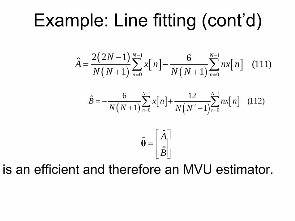
Example: Line fitting (cont’d)

( )( ) [ ] ( ) [ ]

1 1

0 0

2 2 1 6ˆ (111)1 1

N N

n n

NA x n nx n

N N N N

− −

= =

−= −

+ +∑ ∑

( ) [ ] ( ) [ ]1 1

20 0

6 12ˆ (112)1 1

N N

n nB x n nx n

N N N N

− −

= =

= − ++ −∑ ∑

ˆˆ

ˆA

B

⎡ ⎤= ⎢ ⎥⎢ ⎥⎣ ⎦

θ

is an efficient and therefore an MVU estimator.