curs8vniculescu/didactic/curs 8.pdf · acceleraa (“speedup”),% • acceleraa %notatacusp,%...
TRANSCRIPT
Curs 8
Masurarea performantei algoritmilor paraleli
1 Curs 8-‐ PP
General
• Daca in cazul algoritmilor secven;ali performanta este masurata in termenii complexita;ilor ;mp si spa;u, in cazul algoritmilor paraleli se folosesc si alte masuri ale performantei, care au in vedere toate resursele folosite. • Numarul de procesoare in cazul programarii paralele = o resursa importanta
• Pentru compararea corecta a variantei paralele cu cea seriala, trebuie – sa se precizeze arhitectura sistemului de calcul paralel, – sa se aleaga algoritmul serial cel mai bun si – sa se indice daca exista condi;onari ale performantei algoritmului datorita
volumului de date.
2 Curs 8-‐ PP
Observa;i
• In calculul paralel, ob;nerea unui ;mp de execu;e mai bun nu ınseamna neaparat u;lizarea unui numar minim de opera;i, asa cum este ın calculul serial.
• Factorul memorie nu are o importanta foarte mare ın calculul paralel. In schimb, o resursa majora ın ob;nerea unei performante bune a algoritmului paralel o reprezinta numarul de procesoare folosite.
• Daca ;mpul de execu;e a unei opera;i aritme;ce este mult mai mare decat ;mpul de transfer al datelor ıntre doua elemente de procesare, atunci ıntarzierea datorata retelei este nesemnifica;va, dar, ın caz contrar, ;mpul de transfer joaca un rol important ın determinarea performantei programului.
3 Curs 8-‐ PP
4
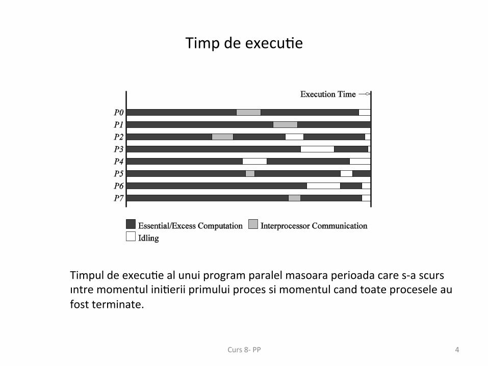
Timp de execu;e
Timpul de execu;e al unui program paralel masoara perioada care s-‐a scurs ıntre momentul ini;erii primului proces si momentul cand toate procesele au fost terminate.
Curs 8-‐ PP
Complexitatea ;mp
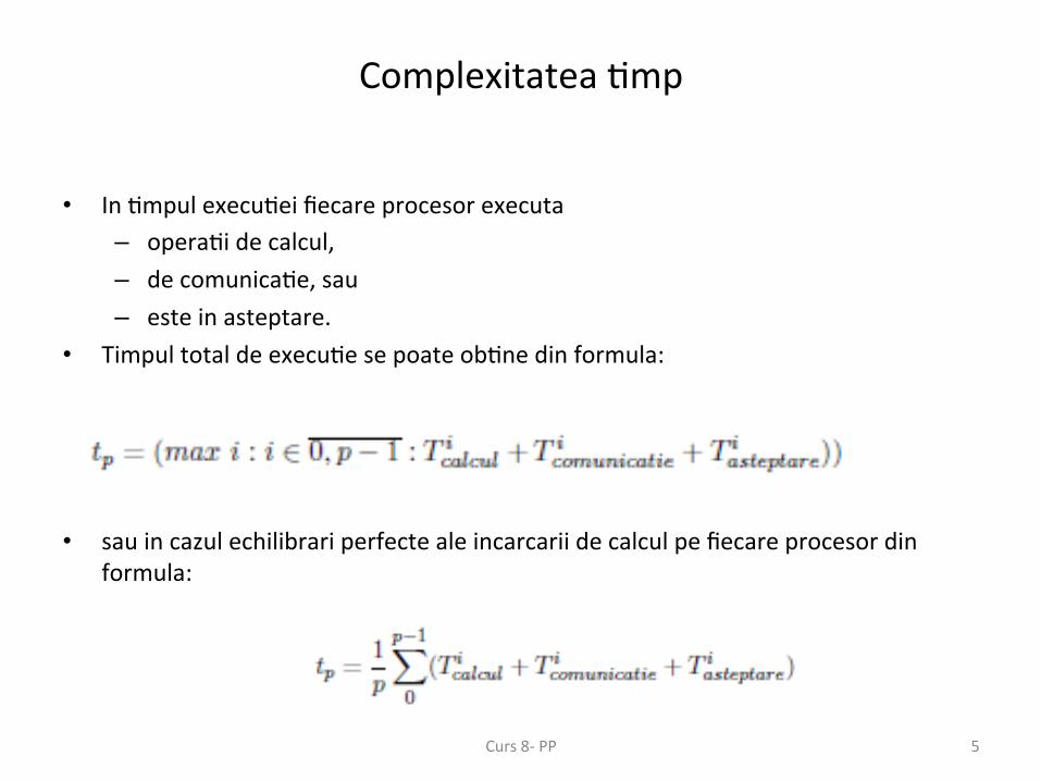
• In ;mpul execu;ei fiecare procesor executa – opera;i de calcul, – de comunica;e, sau – este in asteptare.
• Timpul total de execu;e se poate ob;ne din formula: • sau in cazul echilibrari perfecte ale incarcarii de calcul pe fiecare procesor din
formula:
5 Curs 8-‐ PP
Evaluarea complexita;i
• Ca si in cazul programarii secven;ale, pentru a dezvolta algoritmi paraleli eficien; trebuie sa putem face o evaluare a performantei inca din faza de proiectare a algoritmilor.
• Complexitatea ;mp pentru un algoritm paralel care rezolva o problema Pn cu dimensiunea n a datelor de intrare este o func;e T care depinde de n, dar si de numarul de procesoare p folosite.
• Pentru un algoritm paralel, un pas elementar de calcul se considera a fi o mul;me de opera;i elementare care pot fi executate in paralel de catre o mul;me de procesoare.
• Complexitatea ;mp a unui pas elementar se considera a fi O(1).
• Complexitatea ;mp a unui algoritm paralel este data de numararea atat a pasilor de calcul necesari dar si a pasilor de comunica;e a datelor
6 Curs 8-‐ PP
7
Overhead
• Let Tall be the total ;me collec;vely spent by all the processing elements.
• TS is the serial ;me.
• Tall -‐ TS is the total ;me spend by all processors combined in non-‐goal_computa;on work. This is called the total overhead.
• The total ;me collec;vely spent by all the processing elements
Tall = p TP (p is the number of processors).
• The overhead func;on (To) is therefore given by To = p TP -‐ TS
Curs 8-‐ PP
Accelera;a(“speed-‐up”),
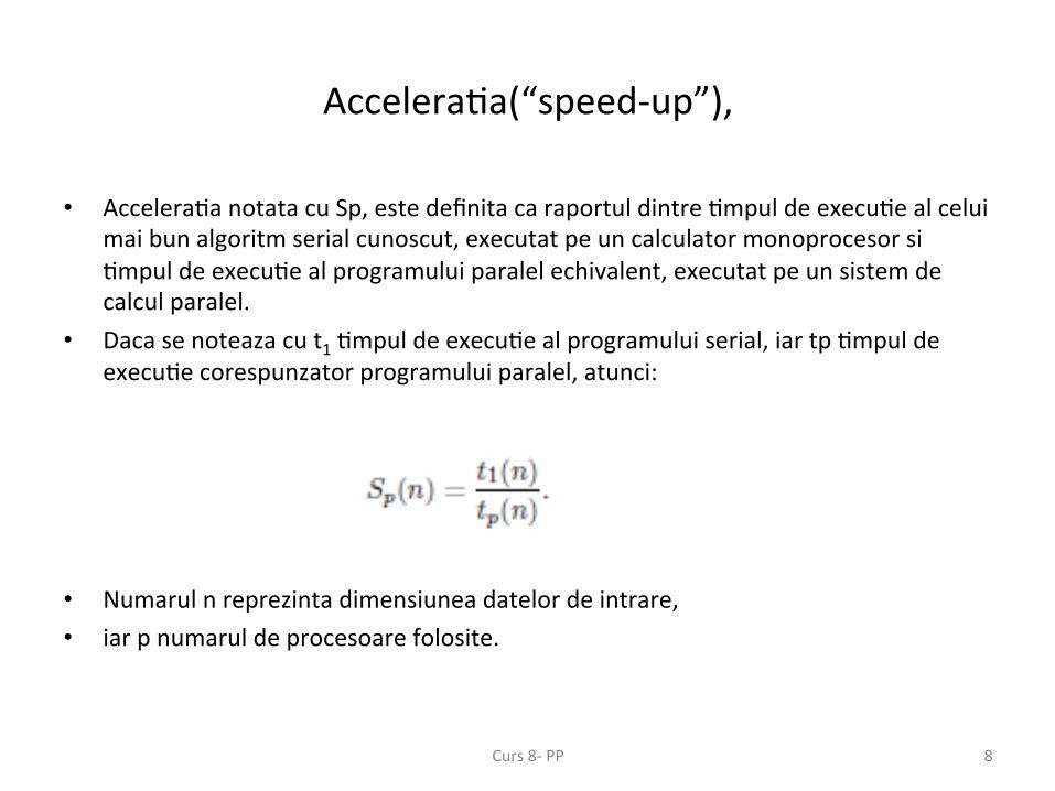
• Accelera;a notata cu Sp, este definita ca raportul dintre ;mpul de execu;e al celui mai bun algoritm serial cunoscut, executat pe un calculator monoprocesor si ;mpul de execu;e al programului paralel echivalent, executat pe un sistem de calcul paralel.
• Daca se noteaza cu t1 ;mpul de execu;e al programului serial, iar tp ;mpul de execu;e corespunzator programului paralel, atunci:
• Numarul n reprezinta dimensiunea datelor de intrare, • iar p numarul de procesoare folosite.
8 Curs 8-‐ PP
Variante
• rela;va, cand ts este ;mpul de execu;e al variantei paralele pe un singur procesor al sistemului paralel;
• reala, cand se compara ;mpul execu;ei paralele cu ;mpul de execu;e pentru varianta
seriala cea mai rapida, pe un procesor al sistemului paralel; • absoluta, cand se compara ;mpul de execu;e al algoritmului paralel cu ;mpul de
execu;e al celui mai rapid algoritm serial, executat de procesorul serial cel mai rapid; • asimpto;ca, cand se compara ;mpul de execu;e al celui mai bun algoritm serial cu
func;a de complexitate asimpto;ca a algoritmului paralel, ın ipoteza existentei numarului necesar de procesoare;
• rela;v asimpto;ca, cand se foloseste complexitatea asimpto;ca a algoritmului paralel executat pe un procesor. Analiza asimpto;ca (considera dimensiunea datelor n si numarul de procesoare p foarte
mari) ignora termenii de ordin mic, si este folositoare ın procesul de construc;e al programelor paralele.
9 Curs 8-‐ PP
Eficienta
• Eficienta este un parametru care masoara gradul de folosire a procesoarelor.
• Eficienta este definita ca fiind:
E = Sp/p • Se deduce ca valoarea eficientei este ıntotdeauna subunitara.
10 Curs 8-‐ PP
Costul
• Costul se defineste ca fiind produsul dintre ;mpul de execu;e si numarul maxim de procesoare care se folosesc.
Cp(n) = tp(n) ·∙ p
• Aceasta defini;e este jus;ficata de faptul ca orice aplica;e paralela poate fi
simulata pe un sistem secven;al, situa;e in care unicul procesor va executa programul intr-‐un ;mp egal cu O(Cp(n)).
• O aplica;e paralela este op(ma din punct de vedere al costului, daca valoarea acestuia este egala, sau este de acelasi ordin de marime cu ;mpul celei mai bune variante secven;ale;
• aplica;a este eficienta din punct de vedere al costului daca Cp = O(t1 log p).
11 Curs 8-‐ PP
“Work”
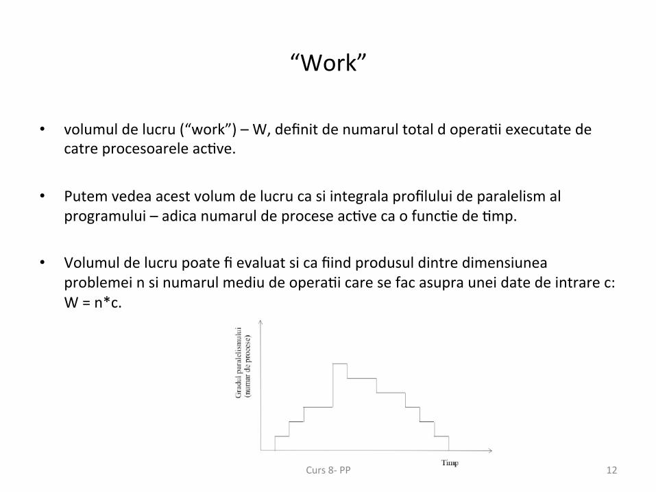
• volumul de lucru (“work”) – W, definit de numarul total d opera;i executate de catre procesoarele ac;ve.
• Putem vedea acest volum de lucru ca si integrala profilului de paralelism al programului – adica numarul de procese ac;ve ca o func;e de ;mp.
• Volumul de lucru poate fi evaluat si ca fiind produsul dintre dimensiunea problemei n si numarul mediu de opera;i care se fac asupra unei date de intrare c: W = n*c.
12 Curs 8-‐ PP
Slide-‐uri engleza -‐ completare
13 Curs 8-‐ PP
14
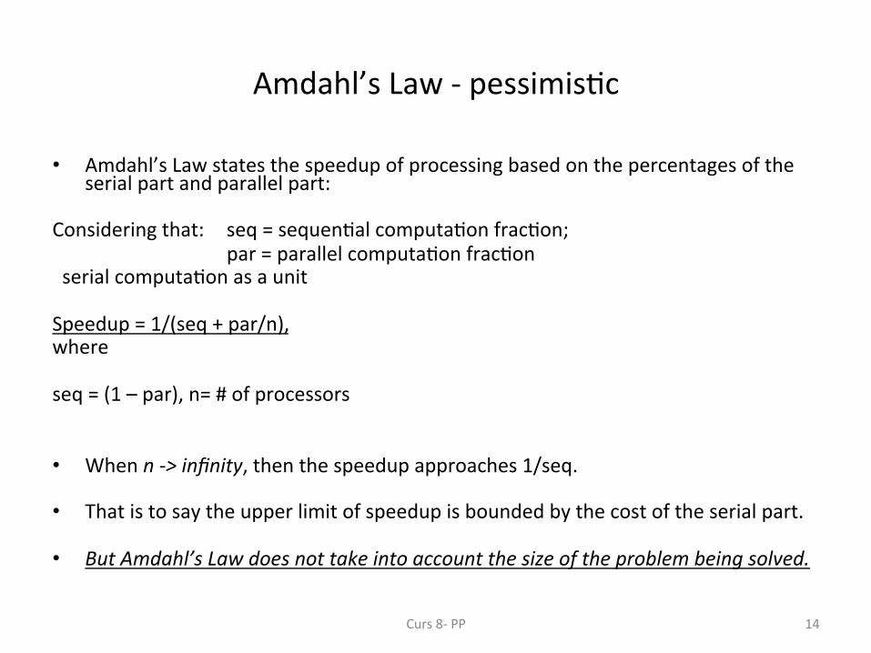
Amdahl’s Law -‐ pessimis;c
• Amdahl’s Law states the speedup of processing based on the percentages of the serial part and parallel part:
Considering that: seq = sequen;al computa;on frac;on;
par = parallel computa;on frac;on serial computa;on as a unit Speedup = 1/(seq + par/n), where seq = (1 – par), n= # of processors • When n -‐> infinity, then the speedup approaches 1/seq. • That is to say the upper limit of speedup is bounded by the cost of the serial part.
• But Amdahl’s Law does not take into account the size of the problem being solved.
Curs 8-‐ PP
15
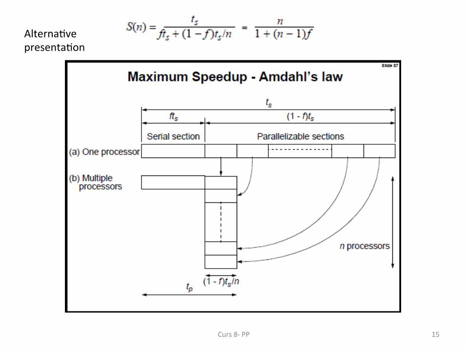
Alterna;ve presenta;on
Curs 8-‐ PP
16
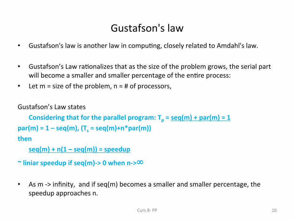
Gustafson's law • Gustafson's law is another law in compu;ng, closely related to Amdahl's law.
• Gustafson’s Law ra;onalizes that as the size of the problem grows, the serial part will become a smaller and smaller percentage of the en;re process:
• Let m = size of the problem, n = # of processors, Gustafson’s Law states
Considering that for the parallel program: Tp = seq(m) + par(m) = 1 par(m) = 1 – seq(m), (Ts = seq(m)+n*par(m)) then
seq(m) + n(1 – seq(m)) = speedup
~ liniar speedup if seq(m)-‐> 0 when n-‐>∞
• As m -‐> infinity, and if seq(m) becomes a smaller and smaller percentage, the speedup approaches n.
Curs 8-‐ PP
17
Gustafson's law -‐ op;mis;c
• In other words, as programs get larger, having mul;ple processors will become more advantageous, and it will get close to n ;mes the performance with n processors as the percentage of the serial part diminishes.
• It assumes the absolute cost of the serial part is constant and does not grow with the size of the problem.
• Amdahl's law assumes a fixed problem size and that the running ;me of the sequen;al sec;on of the program is independent of the number of processors, whereas Gustafson's law does not make these assump;ons.
Curs 8-‐ PP
18
Performance Metrics: Example
• Consider the problem of adding n numbers by using n processing elements.
• If n is a power of two, we can perform this opera;on in log n steps by propaga;ng par;al sums up a logical binary tree of processors.
Curs 8-‐ PP
19
Performance Metrics: Example
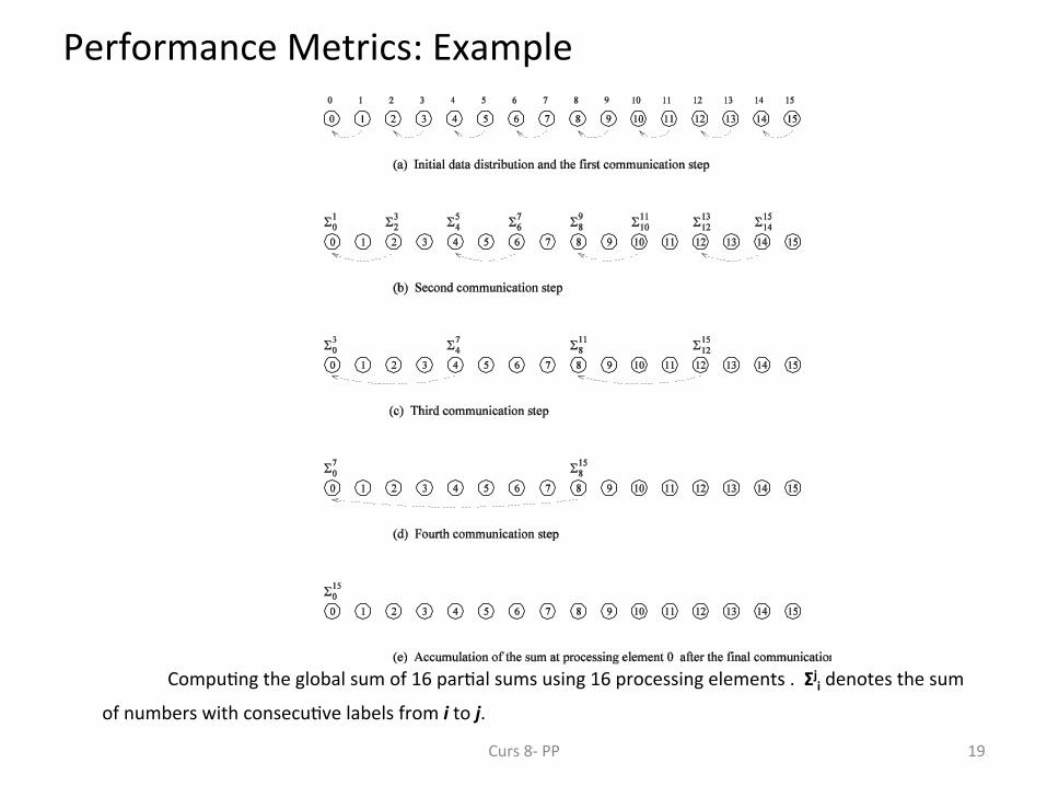
Compu;ng the global sum of 16 par;al sums using 16 processing elements . Σji denotes the sum
of numbers with consecu;ve labels from i to j. Curs 8-‐ PP
20
Performance Metrics: Example (con;nued)
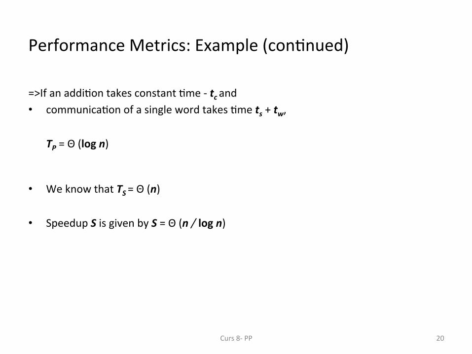
=>If an addi;on takes constant ;me -‐ tc and • communica;on of a single word takes ;me ts + tw,
TP = Θ (log n)
• We know that TS = Θ (n)
• Speedup S is given by S = Θ (n / log n)
Curs 8-‐ PP
21
Performance Metrics: Speedup Bounds
• Speedup can be as low as 0 (the parallel program never terminates).
• Speedup, in theory, should be upper bounded by p – we can only expect a p-‐fold speedup if we use ;mes as many resources.
– A speedup greater than p is possible only if each processing element spends less than ;me TS / p solving the problem.
– In this case, a single processor could be ;me slided to achieve a faster serial program, which contradicts our assump;on of fastest serial program as basis for speedup.
Curs 8-‐ PP
22
Performance Metrics: Superlinear Speedups
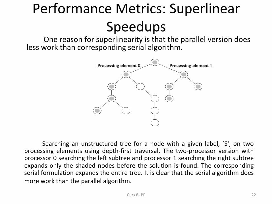
One reason for superlinearity is that the parallel version does less work than corresponding serial algorithm.
Searching an unstructured tree for a node with a given label, `S', on two processing elements using depth-‐first traversal. The two-‐processor version with processor 0 searching the leq subtree and processor 1 searching the right subtree expands only the shaded nodes before the solu;on is found. The corresponding serial formula;on expands the en;re tree. It is clear that the serial algorithm does more work than the parallel algorithm.
Curs 8-‐ PP
23
Performance Metrics: Superlinear Speedups
Resource-‐based superlinearity: The higher aggregate cache/memory bandwidth can result in beser cache-‐hit ra;os, and therefore superlinearity.
Example: A processor with 64KB of cache yields an 80% hit ra;o. If two processors are used, since the problem size/processor is smaller, the hit ra;o goes up to 90%. Of the remaining 10% access, 8% come from local memory and 2% from remote memory.
If DRAM access ;me is 100 ns, cache access ;me is 2 ns, and remote memory access ;me is 400ns, this corresponds to a speedup of 2.43!
Curs 8-‐ PP
24
Parallel Time, Speedup, and Efficiency Example
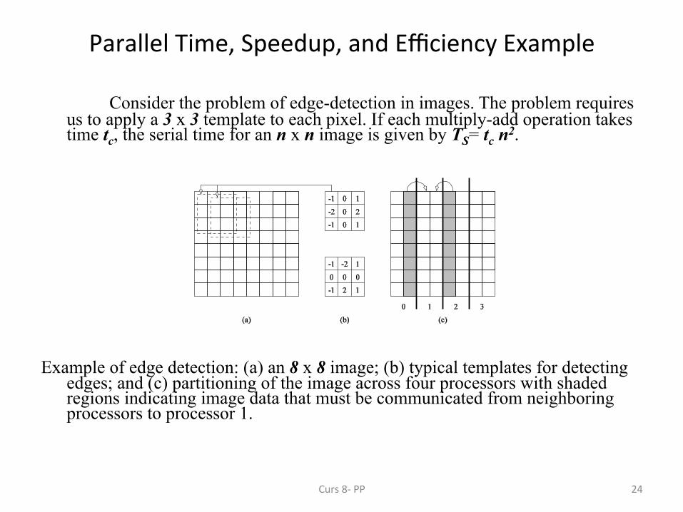
Consider the problem of edge-detection in images. The problem requires us to apply a 3 x 3 template to each pixel. If each multiply-add operation takes time tc, the serial time for an n x n image is given by TS= tc n2.
Example of edge detection: (a) an 8 x 8 image; (b) typical templates for detecting
edges; and (c) partitioning of the image across four processors with shaded regions indicating image data that must be communicated from neighboring processors to processor 1.
Curs 8-‐ PP
25
Parallel Time, Speedup, and Efficiency Example (con;nued)
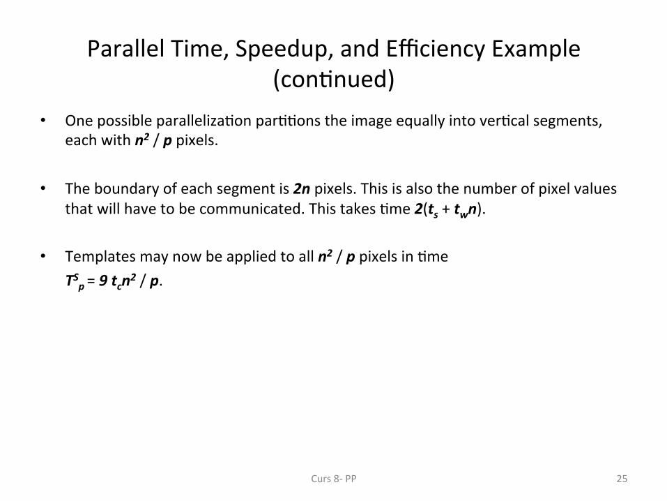
• One possible paralleliza;on par;;ons the image equally into ver;cal segments, each with n2 / p pixels.
• The boundary of each segment is 2n pixels. This is also the number of pixel values that will have to be communicated. This takes ;me 2(ts + twn).
• Templates may now be applied to all n2 / p pixels in ;me TSp = 9 tcn2 / p.
Curs 8-‐ PP
26
Parallel Time, Speedup, and Efficiency Example (con;nued)
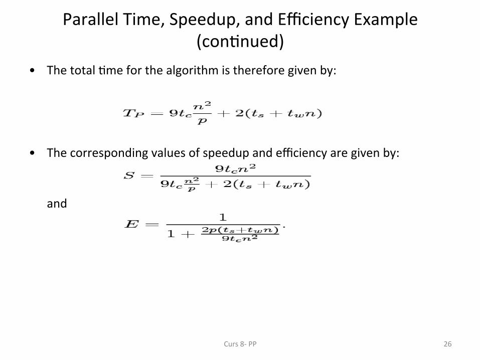
• The total ;me for the algorithm is therefore given by:
• The corresponding values of speedup and efficiency are given by:
and
Curs 8-‐ PP
27
Cost of a Parallel System
• Cost is the product of parallel run;me and the number of processing elements used (p x TP ).
• Cost reflects the sum of the ;me that each processing element spends solving the problem.
• A parallel system is said to be cost-‐opBmal if the cost of solving a problem on a parallel computer is asympto;cally iden;cal to serial cost.
• Since E = TS / p TP, for cost op;mal systems, E = O(1).
• Cost is some;mes referred to as work or processor-‐Bme product.
Curs 8-‐ PP
28
Cost of a Parallel System: Example
Consider the problem of adding numbers on processors. • We have, TP = log n (for p = n).
• The cost of this system is given by p TP = n log n.
• Since the serial run;me of this opera;on is Θ(n), the algorithm is not cost op;mal.
Curs 8-‐ PP
29
Impact of Non-‐Cost Op;mality Consider a sor;ng algorithm that uses n processing elements to sort the list in ;me (log n)2.
• Since the serial run;me of a (comparison-‐based) sort is n log n, the speedup and efficiency of this algorithm are given by n / log n and 1 / log n, respec;vely.
• The p TP product of this algorithm is n (log n)2.
• This algorithm is not cost op;mal but only by a factor of log n.
• If p < n, assigning n tasks to p processors gives TP = n (log n)2 / p .
• The corresponding speedup of this formula;on is p / log n.
• This speedup goes down as the problem size n is increased for a given p !
Curs 8-‐ PP
30
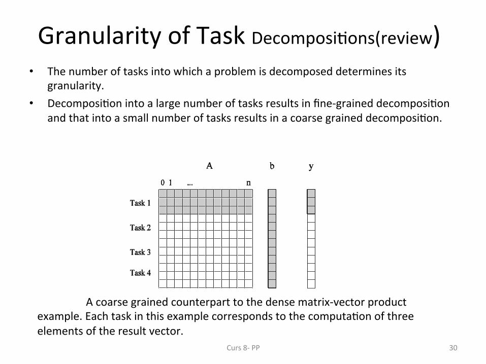
Granularity of Task Decomposi;ons(review) • The number of tasks into which a problem is decomposed determines its
granularity. • Decomposi;on into a large number of tasks results in fine-‐grained decomposi;on
and that into a small number of tasks results in a coarse grained decomposi;on.
A coarse grained counterpart to the dense matrix-‐vector product example. Each task in this example corresponds to the computa;on of three elements of the result vector.
Curs 8-‐ PP
31
Effect of Granularity on Performance
• Oqen, using fewer processors improves performance of parallel systems.
• Using fewer than the maximum possible number of processing elements to execute a parallel algorithm is called scaling down a parallel system.
• A naive way of scaling down is to think of each processor in the original case as a virtual processor and to assign virtual processors equally to scaled down processors.
• Since the number of processing elements decreases by a factor of n / p, the computa;on at each processing element increases by a factor of n / p.
• The communica;on cost should not increase by this factor since some of the virtual processors assigned to a physical processors might talk to each other. This is the basic reason for the improvement from building granularity.
Curs 8-‐ PP
32
Building Granularity: Example
• Consider the problem of adding n numbers on p processing elements such that p < n and both n and p are powers of 2.
• Use the parallel algorithm for n processors, except, in this case, we think of them as virtual processors.
• Each of the p processors is now assigned n / p virtual processors.
• The first log p of the log n steps of the original algorithm are simulated in (n / p) log p steps on p processing elements.
• Subsequent log n -‐ log p steps do not require any communica;on.
Curs 8-‐ PP
33
Building Granularity: Example (con;nued)
• The overall parallel execu;on ;me of this parallel system is Θ ( (n / p) log p).
• The cost is Θ (n log p), which is asympto;cally higher than the Θ (n) cost of adding
n numbers sequen;ally. Therefore, the parallel system is not cost-‐op;mal.
Curs 8-‐ PP
34
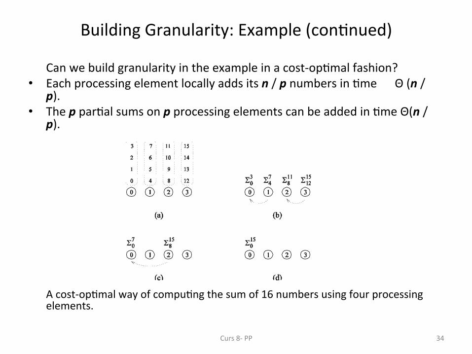
Building Granularity: Example (con;nued)
Can we build granularity in the example in a cost-‐op;mal fashion? • Each processing element locally adds its n / p numbers in ;me Θ (n /
p). • The p par;al sums on p processing elements can be added in ;me Θ(n /
p).
A cost-‐op;mal way of compu;ng the sum of 16 numbers using four processing elements.
Curs 8-‐ PP
35
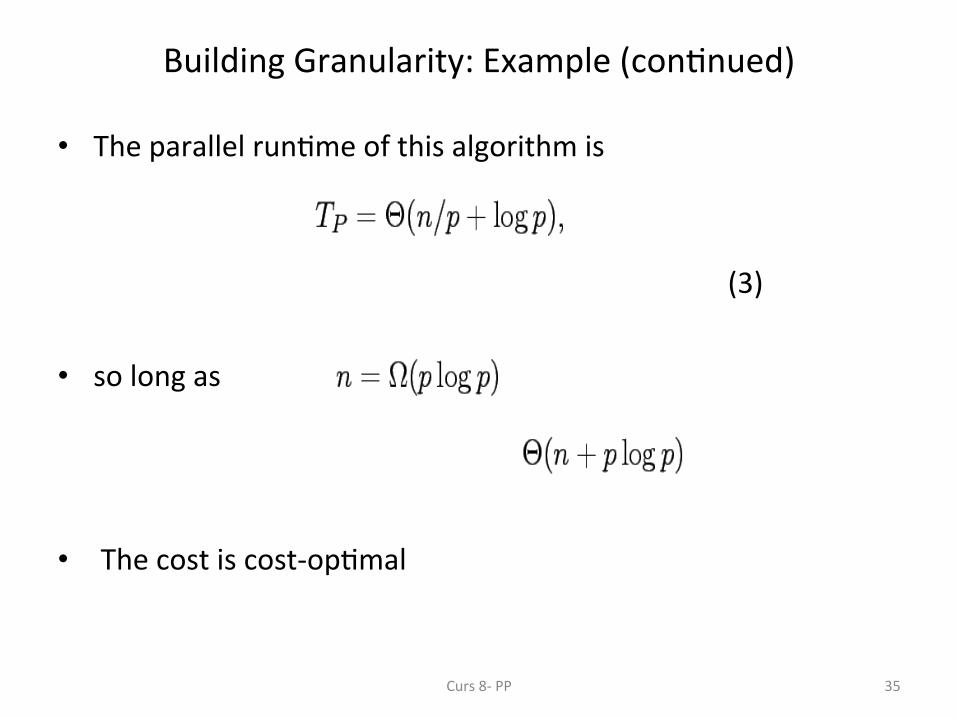
Building Granularity: Example (con;nued)
• The parallel run;me of this algorithm is (3)
• so long as
• The cost is cost-‐op;mal
Curs 8-‐ PP
36
Scalability
• The scalability of parallel system is a measure of its capacity of deliver linear increasing speed-‐up with respect of the number of processors used.
• Scalability analysis is done for a combina;on of an architecture and an algorithm.
• How do we extrapolate performance from small problems and small systems to larger problems on larger configuraBons?
• There are different metrics for scalability –
– the isoefficiency func;on – the Isospeed –efficiency – Serial Frac;on f
Curs 8-‐ PP
37
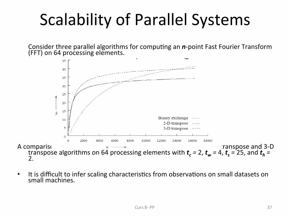
Scalability of Parallel Systems Consider three parallel algorithms for compu;ng an n-‐point Fast Fourier Transform (FFT) on 64 processing elements.
A comparison of the speedups obtained by the binary-‐exchange, 2-‐D transpose and 3-‐D
transpose algorithms on 64 processing elements with tc = 2, tw = 4, ts = 25, and th = 2.
• It is difficult to infer scaling characteris;cs from observa;ons on small datasets on small machines.
Curs 8-‐ PP