buletinul institutului politehnic din iaŞi. mmf 2 din 2016.pdfbuletinul institutului politehnic din...
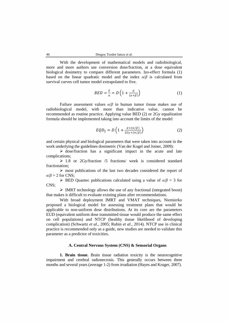
TRANSCRIPT
BULETINUL INSTITUTULUI POLITEHNIC DIN IAŞI
Volumul 62 (66) Numărul 2
Secția MATEMATICĂ. MECANICĂ TEORETICĂ. FIZICĂ 2016 Editura POLITEHNIUM

BULETINUL INSTITUTULUI POLITEHNIC DIN IAŞI PUBLISHED BY
“GHEORGHE ASACHI” TECHNICAL UNIVERSITY OF IAŞI Editorial Office: Bd. D. Mangeron 63, 700050, Iaşi, ROMÂNIA
Tel. 40-232-278683; Fax: 40-232-237666; e-mail: [email protected]
Editorial Board
President: Dan Caşcaval, Rector of the “Gheorghe Asachi” Technical University of Iaşi
Editor-in-Chief: Maria Carmen Loghin, Vice-Rector of the “Gheorghe Asachi” Technical University of Iaşi
Honorary Editors of the Bulletin: Alfred Braier, Mihail Voicu, Corresponding Member of the Romanian Academy,
Carmen Teodosiu
Editors in Chief of the MATHEMATICS. THEORETICAL MECHANICS.
PHYSICS Section
Maricel Agop, Narcisa Apreutesei-Dumitriu, Daniel Condurache
Honorary Editors: Cătălin Gabriel Dumitraş
Associated Editor: Petru Edward Nica
Scientific Board
Sergiu Aizicovici, University “Ohio”, U.S.A. Liviu Leontie, “Al. I. Cuza” University, Iaşi Constantin Băcuţă, Unversity “Delaware”, Newark,
Delaware, U.S.A. Rodica Luca-Tudorache, “Gheorghe Asachi”
Technical University of Iaşi
Masud Caichian, University of Helsinki, Finland Radu Miron, “Al. I. Cuza” University of Iaşi Iuliana Oprea, Colorado State University, U.S.A
Adrian Cordunenu, “Gheorghe Asachi” Technical University of Iaşi
Viorel-Puiu Păun, University “Politehnica” of Bucureşti
Constantin Corduneanu, University of Texas, Arlington, USA.
Lucia Pletea, “Gheorghe Asachi” Technical University of Iaşi
Piergiulio Corsini, University of Udine, Italy Irina Radinschi, “Gheorghe Asachi” Technical University of Iaşi
Sever Dragomir, University “Victoria”, of Melbourne, Australia Themistocles Rassias, University of Athens, Greece
Constantin Fetecău, “Gheorghe Asachi” Technical University of Iaşi
Behzad Djafari Rouhani, University of Texas at El Paso, USA
Cristi Focşa, University of Lille, France Cristina Stan, University “Politehnica” of Bucureşti Wenchang Tan, University “Peking” Beijing, China
Tasawar Hayat, University “Quaid-i-Azam” of Islamabad, Pakistan Petre P. Teodorescu, University of Bucureşti
Radu Ibănescu, “Gheorghe Asachi” Technical University of Iaşi Anca Tureanu, University of Helsinki, Finland
Bogdan Kazmierczak, Inst. of Fundamental Research, Warshaw, Poland
Vitaly Volpert, CNRS, University “Claude Bernard”, Lyon, France

B U L E T I N U L I N S T I T U T U L U I P O L I T E H N I C D I N I A Ş I B U L L E T I N O F T H E P O L Y T E C H N I C I N S T I T U T E O F I A Ş I Volumul 62 (66), Numărul 2 2016
Secția
MATEMATICĂ. MECANICĂ TEORETICĂ. FIZICĂ
Pag.
GRAHAM HALL, Observații asupra clasificării tensorului conform Weyl în varietăți 4-dimensionale de signatură neutră (engl., rez. rom.) . . . . . . .
9
VALERIU POPA și ALINA-MIHAELA PATRICIU, Teoreme de punct fix pentru două perechi de funcţii cu proprietatea limitei comune în spaţii G – metrice (engl., rez. rom.) . . . . . . . . . . . . . . . . . . . . . . . . . . . . . . . . .
19
DRAGOȘ TEODOR IANCU, CAMIL CIPRIAN MIREȘTEAN, CĂLIN GHEORGHE BUZEA, IRINA BUTUC și ALEXANDRU ZARA, Doza totală corelată cu volumul tumoral și riscul de toxicitate în radioterapia modernă (engl., rez. rom.) . . . . . . . . . . . . . . . . . . . . . . . . .
43
CĂLIN GHEORGHE BUZEA, IRINA BUTUC, CAMIL CIPRIAN MIREȘTEAN, ALEXANDRU ZARA și DRAGOȘ TEODOR IANCU, Evaluare dozimetrică comparativă a diferitelor tehnici de radioterapie (3D-CRT, IMRT, VMAT) în tratamentul cancerelor rinosinusale (engl., rez. rom.) . . . . . . . . . . . . . . . . . . . . . . . . . . . . . . . . .
59
CAMIL CIPRIAN MIREȘTEAN, CĂLIN GHEORGHE BUZEA, ALEXANDRU ZARA, IRINA BUTUC și DRAGOȘ TEODOR IANCU, Efectul dozimetric al erorilor sistematice de poziționare prin inducerea artificială a unei deplasări biaxiale de 3 mm a mesei de tratament în radioterapia externă a cancerului de rinofaringe local avansat (engl., rez. rom.) . . . . . . . . . . . . . . . . . . . . . . . . . . . . . . . . . . . . . . .
67
S U M A R

B U L E T I N U L I N S T I T U T U L U I P O L I T E H N I C D I N I A Ş I B U L L E T I N O F T H E P O L Y T E C H N I C I N S T I T U T E O F I A Ş I Volume 62 (66), Number 2 2016
Section
MATHEMATICS. THEORETICAL MECHANICS. PHYSICS
Pp.
GRAHAM HALL, Some Remarks on the Classification of the Weyl Conformal Tensor in 4-Dimensional Manifolds of Neutral Signature (English, Romanian summary) . . . . . . . . . . . . . . . . . . . . . . . . . . . . . . .
9
VALERIU POPA and ALINA-MIHAELA PATRICIU, Fixed Point Theorems for Two Pairs of Mappings Satisfying Common Limit Range Property in G – Metric Spaces (English, Romanian summary) . . . . . . . . . . . . . . .
19
DRAGOȘ TEODOR IANCU, CAMIL CIPRIAN MIREȘTEAN, CĂLIN GHEORGHE BUZEA, IRINA BUTUC and ALEXANDRU ZARA, Total Dose Related to Tumor Volume and Toxicity Risk Correlation in Modern Radiotherapy (English, Romanian summary) . . . . . . . . . . . .
43
CĂLIN GHEORGHE BUZEA, IRINA BUTUC, CAMIL CIPRIAN MIREȘTEAN, ALEXANDRU ZARA and DRAGOȘ TEODOR IANCU, Dosimetric Comparative Evaluation Parameters for Different Radiotherapy Techniques (3D-CRT, IMRT, VMAT) in Paranasal Sinuses Cancers Treatment (English, Romanian summary) . . . . . . . . . .
59
CAMIL CIPRIAN MIREȘTEAN, CĂLIN GHEORGHE BUZEA, ALEXANDRU ZARA, IRINA BUTUC and DRAGOȘ TEODOR IANCU, Dosimetric Influence of Systematic Positioning Errors by Inducing a 3 mm Biaxial Shift in a Case of Locally Advanced Nasopharynx Cancer Treated with External Beam Radiotherapy (English, Romanian summary) . . . . . . . . . . . . . . . . . . . . . . . . . . . . . . . . .
67
C O N T E N T S

BULETINUL INSTITUTULUI POLITEHNIC DIN IAŞI Publicat de
Universitatea Tehnică „Gheorghe Asachi” din Iaşi Volumul 62 (66), Numărul 2, 2016
Secţia MATEMATICĂ. MECANICĂ TEORETICĂ. FIZICĂ
SOME REMARKS ON THE CLASSIFICATION OF THE WEYL CONFORMAL TENSOR IN 4-DIMENSIONAL MANIFOLDS OF
NEUTRAL SIGNATURE
BY
GRAHAM HALL∗
Institute of Mathematics, University of Aberdeen Aberdeen AB24 3UE, Scotland, UK
Received: March 14, 2016 Accepted for publication: August 1, 2016
Abstract. This paper presents a brief discussion of the algebraic
classification of the Weyl conformal tensor on a 4− dimensional manifold with metric g of neutral signature ( , , , )+ + − − . The classification is algebraically similar to the well-known Petrov classification in the Lorentz case and the various algebraic types and corresponding canonical forms are obtained. Further details on principal, totally null 2− spaces and null directions similar to those of L. Bel in the Lorentz case are described.
Keywords: Weyl tensor classification; neutral signature; algebraic structures.
1. Introduction Let M be a 4 − dimensional manifold with smooth metric of neutral
signature ( , , , )+ + − − and let C be the Weyl conformal tensor for ( , )M g . The idea is to provide an algebraic classification of C similar to that given by Petrov in the Lorentz case. The discussion here is brief and more details will be given elsewhere (Hall, 2017). After this work was completed the author was ∗Corresponding author; e-mail: [email protected]
10 Graham Hall
informed that ideas similar to some of those reported here have been given in (Law, 1991; Law, 2006; Batista, 2013; Ortaggio, 2009) and another approach was also presented in (Coley and Hervik, 2010). However, the work here is claimed to be simpler, more structured and to go much further and is more amenable for purposes of calculation.
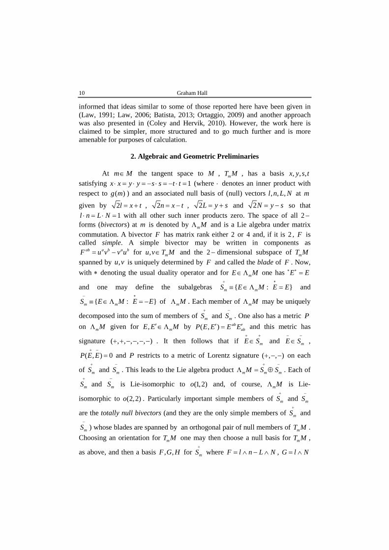
2. Algebraic and Geometric Preliminaries At m M∈ the tangent space to M , mT M , has a basis , , ,x y s t
satisfying 1x x y y s s t t⋅ = ⋅ = − ⋅ = − ⋅ = (where ⋅ denotes an inner product with respect to ( )g m ) and an associated null basis of (null) vectors , , ,l n L N at m
given by 2l x t= + , 2n x t= − , 2L y s= + and 2N y s= − so that 1l n L N⋅ = ⋅ = with all other such inner products zero. The space of all 2 −
forms (bivectors) at m is denoted by mMΛ and is a Lie algebra under matrix commutation. A bivector F has matrix rank either 2 or 4 and, if it is 2 , F is called simple. A simple bivector may be written in components as
ab a b a bF u v v u= − for , mu v T M∈ and the 2 − dimensional subspace of mT M spanned by ,u v is uniquely determined by F and called the blade of F . Now, with ∗ denoting the usual duality operator and for mE M∈Λ one has E E∗ ∗ =
and one may define the subalgebras { : }m mS E M E E+ ∗
≡ ∈Λ = and
{ : }m mS E M E E− ∗
≡ ∈Λ = − of mMΛ . Each member of mMΛ may be uniquely
decomposed into the sum of members of mS+
and mS−
. One also has a metric P on mMΛ given for , mE E M′∈Λ by ( , ) ab
abP E E E E′ ′= and this metric has
signature ( , , , , , )+ + − − − − . It then follows that if mE S+ +
∈ and mE S− −
∈ ,
( , ) 0P E E+ −
= and P restricts to a metric of Lorentz signature ( , , )+ − − on each
of mS+
and mS−
. This leads to the Lie algebra product m m mM S S+ −
Λ = ⊕ . Each of
mS+
and mS−
is Lie-isomorphic to (1,2)o and, of course, mMΛ is Lie-
isomorphic to (2,2)o . Particularly important simple members of mS+
and mS−
are the totally null bivectors (and they are the only simple members of mS+
and
mS−
) whose blades are spanned by an orthogonal pair of null members of mT M . Choosing an orientation for mT M one may then choose a null basis for mT M ,
as above, and then a basis , ,F G H for mS+
where F l n L N= ∧ − ∧ , G l N= ∧
Bul. Inst. Polit. Iaşi, Vol. 62 (66), Nr. 2, 2016 11
and H n L= ∧ (and similarly F l n L N−
= ∧ + ∧ , G l L−
= ∧ and H n N−
= ∧ is a
basis for mS−
). In these bases G and H are totally null members of mS+
and G−
and H−
are totally null members of mS−
.
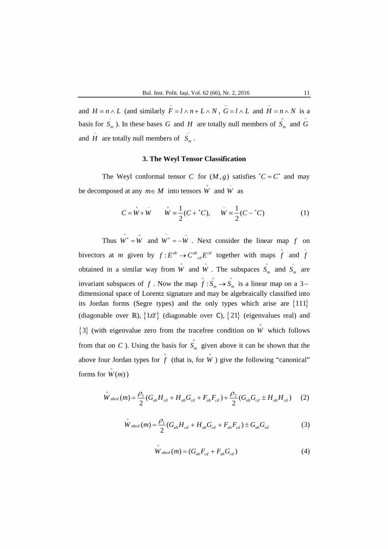
3. The Weyl Tensor Classification The Weyl conformal tensor C for ( , )M g satisfies C C∗ ∗= and may
be decomposed at any m M∈ into tensors W+
and W−
as
1 1 ( ), ( )2 2
C W W W C C W C C+ − + −
∗ ∗= + ≡ + ≡ − (1)
Thus W W+ +∗ = and W W
− −∗ = − . Next consider the linear map f on
bivectors at m given by : ab ab cdcdf E C E→ together with maps f
+
and f−
obtained in a similar way from W+
and W−
. The subspaces mS+
and mS−
are
invariant subspaces of f . Now the map : m mf S S+ + +
→ is a linear map on a 3−dimensional space of Lorentz signature and may be algebraically classified into its Jordan forms (Segre types) and the only types which arise are { }111
(diagonable over ℝ), { }1zz (diagonable over ℂ), { }21 (eigenvalues real) and
{ }3 (with eigenvalue zero from the tracefree condition on W+
which follows
from that on C ). Using the basis for mS+
given above it can be shown that the
above four Jordan types for f+
(that is, for W+
) give the following “canonical”
forms for ( )W m+
)
1 2( ) ( ) ( )2 2
abcd ab cd ab cd ab cd ab cd ab cdW m G H H G F F G G H Hρ ρ+
= + + + ± (2)
1( ) ( )2
abcd ab cd ab cd ab cd ab cdW m G H H G F F G Gρ+
= + + ± (3)
( ) ( )abcd ab cd ab cdW m G F F G+
= + (4)
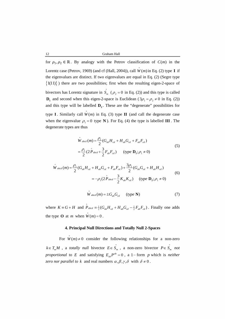
12 Graham Hall
for 𝜌𝜌1,𝜌𝜌2 ∈ ℝ . By analogy with the Petrov classification of ( )C m in the
Lorentz case (Petrov, 1969) (and cf (Hall, 2004)), call ( )W m+
in Eq. (2) type I if the eigenvalues are distinct. If two eigenvalues are equal in Eq. (2) (Segre type { }1(11) ) there are two possibilities; first when the resulting eigen-2-space of
bivectors has Lorentz signature in mS+
( 2 0ρ = in Eq. (2)) and this type is called
1D and second when this eigen-2-space is Euclidean ( 1 23 0ρ ρ= ≠ in Eq. (2)) and this type will be labelled 2D . These are the “degenerate” possibilities for
type I . Similarly call ( )W m+
in Eq. (3) type II (and call the degenerate case when the eigenvalue 1 0ρ = type N ). For Eq. (4) the type is labelled III . The degenerate types are thus
1
11
( ) ( )2
3(2 ) ( ; 0)2 2
abcd ab cd ab cd ab cd
abcd ab cd
W m G H H G F F
P F F type
ρ
ρ ρ
+
+
= + +
= + ≠1D (5)
1 1
1 1
3( ) ( ) ( )2 2
3 (2 ) ( ; 0)2
abcd ab cd ab cd ab cd ab cd ab cd
abcd ab cd
W m G H H G F F G G H H
P K K type
ρ ρ
ρ ρ
+
+
= + + + +
= − − ≠2D (6)
( ) ( )abcd ab cdW m G G type+
= ± N (7)
where K G H≡ + and 1 12 2( )abcd ab cd ab cd ab cdP G H H G F F
+
≡ + − . Finally one adds
the type O at m when ( ) 0W m+
= .
4. Principal Null Directions and Totally Null 2-Spaces
For ( ) 0W m+
≠ consider the following relationships for a non-zero
mk T M∈ , a totally null bivector mE S+
∈ , a non-zero bivector mP S+
∈ not
proportional to E and satisfying 0ababE P = , a 1− form p which is neither
zero nor parallel to k and real numbers , , ,α β γ δ with 0δ ≠ .
Bul. Inst. Polit. Iaşi, Vol. 62 (66), Nr. 2, 2016 13
( ) , ( ) b d cdabcd abcda c abi W k k k k ii W E Eα β
+ +
= = (8)
( ) ( ) b d cdabcd abcda c a c ab abi W k k k p p k ii W E E Pγ δ
+ +
= + = + (9)
The vector k in Eq. (8(i)) is necessarily null and will be said to span a
repeated principal null direction of ( )W m+
(a repeated pnd) (cf (Bel, 2000; Sachs, 1961; Hall, 2004)). The blade of the totally null bivector E in Eq. (8(ii)) will be called a repeated principal totally null 2 − space (a repeated 2 − space)
of ( )W m+
(and E is an eigenbivector of ( )W m+
). The vector k in Eq. (9(i)) can be shown to be necessarily null and will be said to span a general principal null
direction of ( )W m+
(a general pnd) [and a set of equivalent conditions on k are
(i) that ] [[ ] 0a bc db c
e fk W k k k+
= where square brackets denote the usual skew-symmetrisation of indices, and (ii) that Eq. (8(i)) is false]. Collectively, repeated and general pnds will be referred to simply as pnds. The blade of the bivector E in Eq. (9(ii)) will be called a general principal totally null 2 − space (a
general 2 − space) of ( )W m+
. Collectively, repeated and general such 2 − spaces
are called principal 2 − spaces of ( )W m+
. Assuming that ( ) 0W m+
≠ the following hold;
Lemma 1
(i) There exists 0 mk T M≠ ∈ such that 0dabcdW k
+
= if and only if
( )W m+
is type N . The vector k spans a repeated pnd and may be any non-zero member of the totally null blade of the bivector G in Eq. (7) (and only these).
The bivector G is the unique totally null member of mS+
(up to a scaling) satisfying Eq. (8(ii)) and, in fact, 0β = .
(ii) There exists 0 mk T M≠ ∈ such that 0b dabcdW k k
+
= if and only if
( )W m+
is type N or III . Again k spans a repeated pnd and may be any non-zero member of the totally null blade of the bivector G in Eq. (7) or Eq. (4)
(and only these). The bivector G is the unique totally null member of mS+
(up to a scaling) satisfying Eq. (8(ii)) and, in fact, 0β = .
14 Graham Hall
(iii) There exists 0 mk T M≠ ∈ such that b dabcd a cW k k k kα
+
= with
0 ≠ 𝛼𝛼 ∈ ℝ if and only if ( )W m+
is type II or 1D . Again k spans a repeated pnd and may be any non-zero member of the totally null blade of the bivector G in Eq. (3) for type II (and only these), or any member of the totally null blades of G and H in Eq. (5) for 1D (and only these). The bivectors G (for type II ) and G and H (for type 1D ) are the unique totally null member(s) of
mS+
(up to a scaling) satisfying Eq. (8(ii)) and in all cases 0β α≠ ≠ with the same β arising for both G and H and the same α for the associated pnds in type 1D .
(iv) If there exists 0 mk T M≠ ∈ such that Eq. (9(i)) holds then k spans a general pnd and may be any member of the totally null blade of a bivector
mE S+
∈ satisfying Eq. (9(ii)). The non-zero members of the blade of any totally
null mE S+
∈ satisfying Eq. (9(ii)) span general pnds.
Thus finding repeated pnds for ( )W m+
amounts to finding its totally null eigenbivectors E as in Eq. (8(ii)). If such an eigenbivector exists either it is
unique (up to a scaling) and then the type of ( )W m+
is N , III ( 0β α= = in Eq. (8)) or II ( 0β α≠ ≠ in Eq. (8)) or two independent such eigenbivectors exist each with the same eigenvalue 0β ≠ ( 0α⇒ ≠ ) in Eq. (8) and then the type is
1D . The finding of general pnds amounts to solving Eq. (9(ii)) for E and is perhaps more conveniently done by writing this latter equation in the equivalent
form 0ab cdabcdW E E
+
= with E not an eigenbivector of W+
. This last equation results in a polynomial equation of order at most 4 for real solutions for E . Such solutions can then be calculated from Eq. (2)-Eq. (7). The resulting set of (real) solutions gives the complete set of solutions for principal 2 − spaces and
pnds (repeated pnds arising if E is an eigenbivector of W+
and general pnds otherwise) and these solutions can be shown to justify the term “repeated”. It is remarked here that “real” solutions are required. This is because the general solutions of these polynomials sometimes contain complex totally null bivectors as solutions. The blades of such solutions actually contain no non-zero real vectors (up to scaling) and are thus rejected in this analysis (Hall, 2016).
Of course, similar results apply to W−
and mS−
and the repeated and general pnds collectively give a description of C . To see this consider the
Bul. Inst. Polit. Iaşi, Vol. 62 (66), Nr. 2, 2016 15
following equations for ( )C m , for a non-zero mk T M∈ , for a 1− form p at m which is neither zero nor parallel to k and with 𝛼𝛼 ∈ ℝ .
( ) ( ) b d b dabcd a c abcd a c a ci C k k k k ii C k k k p p kα= = + (10)
If 0α ≠ in (i), k is necessarily null but this is not true if 0α = (see
(Hall, 2017; Hall, 2016)). So suppose that Eq. (10(i)) holds with k assumed null. Then k is said to span a repeated principal null direction of ( )C m (a repeated pnd). If Eq. (10(ii)) holds, k is necessarily null (and orthogonal to p ) and is said to span a general principal null direction of ( )C m (a general pnd).
[A set of equivalent statements to Eq. (10(ii)) are that ( )a [ ] [ ] 0b ce a bc d fk C k k k =
at m and ( )b that Eq. (10(i)) is false]. Collectively, repeated and general pnds of C are referred to as pnds of C . Such directions are related to the analogous
ones for W+
and W−
by the following lemma.
Lemma 2 A vector mk T M∈ spans a repeated pnd for C if and only if it spans a
repeated pnd for W+
and W−
. A vector mk T M∈ spans a general pnd for C if
and only if it spans a pnd for W+
and W−
and is general for at least one of them. It is noted and easily shown that any real eigenbivector of ( )C m is
either a member of mS+
or mS−
or, if not, lies in an eigenspace of C spanned by
eigenbivectors in mS+
or mS−
. Thus one may think of all the eigenbivectors of C
as being in mS+
or mS−
. In fact, a canonical form for ( )C m is obtained from Eq.
(1) by simply adding together canonical forms for ( )W m+
and ( )W m−
and the
Segre type of ( )C m is simply the “sum” of the Segre types of ( )W m+
and ( )W m−
(with any brackets denoting degeneracies appropriately inserted). To determine the pnds of ( )C m one notes the following easily checked result that the
intersection of two totally null 2 − spaces each of which lies in mS+
or each of
which lies in mS−
is just the trivial subspace whereas the intersection of two
totally null 2 − spaces one of which lies in mS+
and the other in mS−
is a null
16 Graham Hall
direction at m . Thus when the principal 2 − spaces of ( )W m+
and ( )W m−
are
known (and which lie, respectively, in mS+
and mS−
) their intersections give the pnds of ( )C m according to lemma 2. The algebraic type of ( )C m can then be
labelled ( , )A B where A and B are the algebraic types for ( )W m+
and ( )W m−
. For example, ( )C m has type ( , )N N if and only if there exists a unique null direction spanned by k at m satisfying 0d
abcdC k = and which is the
intersection of the (unique) repeated principal 2 − spaces for ( )W m+
and ( )W m−
for type N . A consequence of this classification is the fact that there are finitely
many (real) principal 2 − spaces for ( )W m+
and ( )W m−
(possibly none---see an earlier remark) and hence finitely many pnds for ( )C m (possibly none) except when the latter's algebraic type is of the form ( , )A O for certain choices of A (e.g., type ( , )N O ) when infinitely many pnds occur.
Of course, the above classification is pointwise on M . However, one can display a topological decomposition of (an open dense subset of) M into
open subsets of M on which the algebraic types of W+
, W−
and C are constant. Also one can demonstrate the local smoothness (in an obvious sense) of the canonical forms and decompositions described in section 3 as well as study the isotropies arising from the the tetrad changes which preserve the given
canonical forms for W+
, W−
and C . This will be published elsewhere (Hall, 2017). In this last respect the study of the subalgebra structure of (2,2)o given in (Ghanam and Thompson, 2001) and, in a more accessible form for the present purposes in (Wang and Hall, 2013), is useful.
Acknowledgements. The author wishes to thank the organisers of the International Conference on Applied and Pure Mathematics (ICAPM 2015) in Iași, Romania, for their invitation to him to lecture at this meeting and for their hospitality. This paper is the text of that lecture. He also thanks Cornelia-Livia Bejan and her colleagues for their many kindnesses throughout his stay in Iași.
REFERENCES Batista C., Weyl Tensor Classification in Four-Dimensional Manifolds of All
Signatures, arXiv: 1204.5133v4 (2013). Bel L., Radiation States and the Problem of Energy in General Relativity, Gen. Rel.
Grav., 30, 2047 (2000) (This is an English translation of the original paper Cah. Phys., 16, 59 (1962)).
Bul. Inst. Polit. Iaşi, Vol. 62 (66), Nr. 2, 2016 17
Coley A., Hervik S., Higher Dimensional Bivectors and Classification of the Weyl Operator, Class. Quant. Grav., 27, 015002 (2010).
Ghanam R., Thompson G., The Holonomy Lie Algebras of Neutral Metrics in Dimension Four, J. Math. Phys., 42, 2266 (2001).
Hall G.S., Symmetries and Curvature Structure in General Relativity, World Scientific (2004).
Hall G.S., Some Comparisons of the Weyl Conformal Tensor and Its Classification in 4-Dimensional Lorentz, Neutral and Positive Definite Signatures, Preprint, University of Aberdeen (2016).
Hall G.S., The Classification of the Weyl Conformal Tensor in 4-Dimensional Manifolds of Neutral Signature, J. Geom. Phys., 111, 111-125 (2017).
Law P., Neutral Einstein Metrics in Four Dimensions, J. Math. Phys., 32, 3039-3042 (1991).
Law P., Classification of the Weyl Curvature Spinors of Neutral Metrics in Four Dimensions, J. Geom. Phys., 56, 2093-2018 (2006).
Ortaggio M., Bel-Debever Criteria for the Classification of the Weyl Tensor in Higher Dimensions, Class. Quant. Grav., 26, 195015 (2009).
Petrov A.Z., Einstein Spaces, Pergamon (1969). Sachs R.K., Gravitational Waves in General Relativity, VI: The Outgoing Radiation
Condition, Proc. Roy. Soc., A264, 309 (1961). Wang Z., Hall G.S., Projective Structure in 4-Dimensional Manifolds with Metric
Signature ( , , , )+ + − − , J. Geom. Phys., 66, 37-49 (2013).
OBSERVAȚII ASUPRA CLASIFICĂRII TENSORULUI CONFORM WEYL ÎN VARIETĂȚI 4-DIMENSIONALE
DE SIGNATURĂ NEUTRĂ
(Rezumat)
Această lucrare prezintă o scurtă discuție asupra clasificării algebrice a tensorului conform Weyl pe o varietate 4-dimensională cu metrică g de signatură neutră (+,+,-,-). Din punct de vedere algebric, clasificarea este similară cu binecunoscuta clasificare Petrov în cazul Lorentz. Sunt obținute diferite tipuri algebrice și formele canonice corespunzătoare. Sunt descrise mai multe detalii ale 2-spațiilor principale total nule și ale direcțiilor nule, similare celor ale lui L. Bel din cazul Lorentz.

BULETINUL INSTITUTULUI POLITEHNIC DIN IAŞI Publicat de
Universitatea Tehnică „Gheorghe Asachi” din Iaşi Volumul 62 (66), Numărul 2, 2016
Secţia MATEMATICĂ. MECANICĂ TEORETICĂ. FIZICĂ
FIXED POINT THEOREMS FOR TWO PAIRS OF MAPPINGS SATISFYING COMMON LIMIT RANGE PROPERTY IN
G – METRIC SPACES
BY
VALERIU POPA1 and ALINA-MIHAELA PATRICIU2,*
1 “Vasile Alecsandri” University of Bacău 2 “Dunărea de Jos” University of Galaţi, Faculty of Sciences and Environment,
Department of Mathematics and Computer Sciences
Received: February 12, 2016 Accepted for publication: August 31, 2016
Abstract. The purpose of this paper is to prove a general fixed point
theorem for two pairs of mappings in G - metric spaces, generalizing the results from (Popa and Patriciu, 2014) and unifying the results from (Giniswamy and Maheshwari, 2014). Also, a new result for a sequence of mappings is obtained. In the last part of this paper as applications, some fixed point results for mappings satisfying contractive conditions of integral type, for almost contractive mappings, for φ - contractive mappings and ),( ψφ - contractive mappings in G - metric spaces, are obtained.
Keywords: fixed point; almost altering distance; common limit range property; implicit relation; G - metric space.
1. Introduction
Let ),( dX be a metric space and TS , be two mappings of X . In
1996, Jungck (Jungck, 1996) defined S and T to be compatible if *Corresponding author; e-mail: [email protected]
Valeriu Popa and Alina-Mihaela Patriciu
20
0=),(lim nnn
STxTSxd∞→
whenever }{ nx is a sequence in X such that
,=lim=lim tTxSx n
nn
n ∞→∞→
for some Xt ∈ .
This concept has been frequently used to prove the existence theorems in fixed point theory.
Let gf , be self mappings of a nonempty set X . A point Xx∈ is a coincidence point of f and g if gxfxw == and w is said to be a point of coincidence of f and g . The set of all coincidence points of f and g is denoted by ),( gfC .
In 1994, Pant (Pant, 1994) introduced the notion of pointwise R - weakly commuting mapping, which is equivalent to commutativity at coincidence points.
In 1996, Jungck (Jungck, 1996) introduced the notion of weakly compatible mappings.
Definition 1.1 (Jungck, 1996) Let X be a nonempty set and gf , be self mappings of X . f and g are weakly compatible if gfufgu = for all
),( gfCu∈ . Hence, f and g are weakly compatible if and only if f and g are
pointwise R - weakly commuting. The study of common fixed points for noncompatible mappings is also
interesting, the work of this regard beeing initiated by Pant in (Pant, 1998; 1999).
Aamri and El - Moutawakil (2002) introduced a generalization of noncompatible mappings.
Definition 1.2 (Aamri and El - Moutawakil, 2002) Let S and T be two self mappings of a metric space ( )dX , . We say that S and T satisfy property ( )EA if there exists a sequence }{ nx in X such that
,=lim=lim tSxTx nn
nn ∞→∞→
for some Xt ∈ . Remark 1.1 It is clear that two self mappings S and T of a metric
space ( )dX , will be noncompatible if there exists }{ nx in X such that tTxSx nnnn =lim=lim ∞→∞→ , for some Xt ∈ but ),(lim nnn TSxSTxd∞→ is
non zero or non existent.
Bul. Inst. Polit. Iaşi, Vol. 62 (66), Nr. 2, 2016 21
Therefore, two noncompatible self mappings of a metric space ( )dX , satisfy property ( )EA .
It is known from (Pathak et al., 2010) that the notions of weakly compatible mappings and mappings satisfying property ( )EA are independent.
There exists a vast literature concerning the study of fixed points for pairs of mappings satisfying property ( )EA .
In 2005, Liu et al. (Liu et al., 2005) defined the notion of common property ( )EA .
Definition 1.3 (Liu et al., 2005) Two pairs ( )SA, and ( )TB, of self mappings of a metric space ( )dX , are said to satisfy common property ( )EA if there exist two sequences }{ nx and }{ ny in X such that
,=lim=lim=lim=lim tTyBySxAx nn
nn
nn
nn ∞→∞→∞→∞→
for some Xt ∈ . In 2011, Sintunavarat and Kumam (Sintunavarat and Kumam, 2011)
introduced the notion of common limit range property. Definition 1.4 (Sintunavarat and Kumam, 2011) A pair ( )SA, of self
mappings of a metric space ( )dX , is said to satisfy the common limit range property with respect to S , denoted )(SCLR if there exists a sequence }{ nx in X such that
,=lim=lim tSxAx nn
nn ∞→∞→
for some )(XSt∈ . Thus we can infer that a pair ( )SA, satisfying the property ( )EA along
with the closedness of the subspace ( )XS always has the )(SCLR - property with respect to S (see Examples 2.16, 2.17 (Imdad et al., 2012)).
Recently, Imdad et al. (2013) extended the notion of common limit range property to the pairs of self mappings.
Definition 1.5 (Imdad et al., 2013) Two pairs ( )SA, and ( )TB, of self mappings of a metric space ( )dX , are said to satisfy common limit range property with respect to S and T , denoted ),( TSCLR if there exist two sequences }{ nx and }{ ny in X such that
,=lim=lim=lim=lim tTyBySxAx nn
nn
nn
nn ∞→∞→∞→∞→
where ( )XTXSt ∩∈ )( . Some fixed point results for pairs of mappings with ),( TSCLR property are
obtained in (Imdad and Chauhan, 2013; Karapinar et al., 2013) and in other papers.
Valeriu Popa and Alina-Mihaela Patriciu
22
2. Preliminaries
In (Dhage, 1992; 2000), Dhage introduced a new class of generalized metric space, named D - metric spaces. Mustafa and Sims (2003; 2006), proved that most of the claims concerning the fundamental topological structures on D - metric spaces are incorrect and introduced appropriate notion of generalized metric space, named G - metric space. In fact, Mustafa, Sims and other authors studied many fixed point results for self mappings under certain conditions in (Mustafa et al., 2008; Mustafa and Sims, 2009; Shatanawi, 2010), and in other papers.
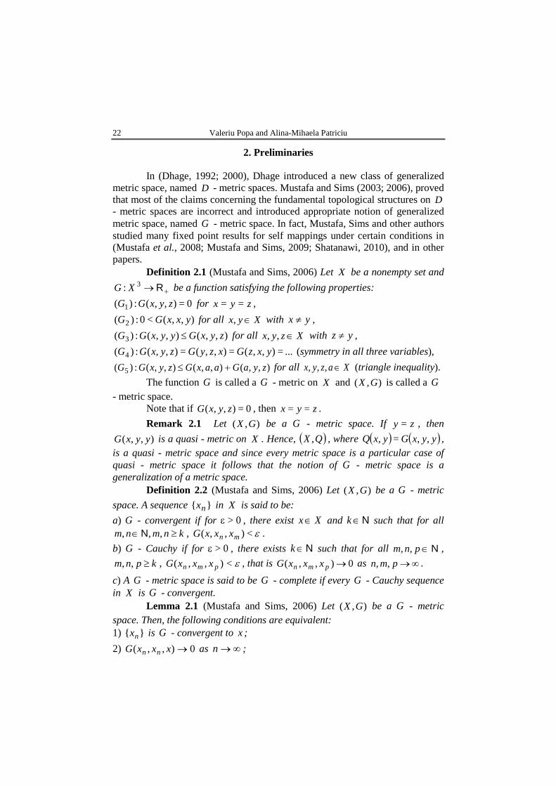
Definition 2.1 (Mustafa and Sims, 2006) Let X be a nonempty set and
+→ R3: XG be a function satisfying the following properties: 0=),,(:)( 1 zyxGG for zyx == , ),,(<0:)( 2 yxxGG for all Xyx ∈, with yx ≠ ,
),,(),,(:)( 3 zyxGyyxGG ≤ for all Xzyx ∈,, with yz ≠ , ...=),,(=),,(=),,(:)( 4 yxzGxzyGzyxGG (symmetry in all three variables),
),,(),,(),,(:)( 5 zyaGaaxGzyxGG +≤ for all Xazyx ∈,,, (triangle inequality). The function G is called a G - metric on X and ),( GX is called a G
- metric space. Note that if 0=),,( zyxG , then zyx == . Remark 2.1 Let ),( GX be a G - metric space. If zy = , then ),,( yyxG is a quasi - metric on X . Hence, ( )QX , , where ( ) ( )yyxGyxQ ,,=, ,
is a quasi - metric space and since every metric space is a particular case of quasi - metric space it follows that the notion of G - metric space is a generalization of a metric space.
Definition 2.2 (Mustafa and Sims, 2006) Let ),( GX be a G - metric space. A sequence }{ nx in X is said to be: a) G - convergent if for 0>ε , there exist Xx∈ and N∈k such that for all
knmnm ≥∈ ,,, N , ε<),,( mn xxxG . b) G - Cauchy if for 0>ε , there exists N∈k such that for all N∈pnm ,, ,
kpnm ≥,, , ε<),,( pmn xxxG , that is 0),,( →pmn xxxG as ∞→pmn ,, . c) A G - metric space is said to be G - complete if every G - Cauchy sequence in X is G - convergent.
Lemma 2.1 (Mustafa and Sims, 2006) Let ),( GX be a G - metric space. Then, the following conditions are equivalent: 1) }{ nx is G - convergent to x ; 2) 0),,( →xxxG nn as ∞→n ;
Bul. Inst. Polit. Iaşi, Vol. 62 (66), Nr. 2, 2016 23
3) 0),,( →xxxG n as ∞→n ; 4) 0),,( →xxxG mn as ∞→mn, .
Lemma 2.2 (Mustafa and Sims, 2006) If ),( GX is a G - metric space, then the following conditions are equivalent: 1) }{ nx is G - Cauchy; 2) For 0>ε , there exists N∈k such that ε<),,( mmn xxxG for all N∈nm, ,
knm ≥, . Lemma 2.3 (Mustafa and Sims, 2006) Let ),( GX be a G - metric
space. Then, the function ),,( zyxG is jointly continuous in all three of its variables.
Definition 2.3 (Mustafa and Sims, 2006) A G - metric on a set X is said to be symmetric if ( ) ( )xxyGyyxG ,,=,, for all Xyx ∈, . Then, ( )GX , is said to be symmetric G - metric space.
Quite recently (Popa and Patriciu, 2014), a general fixed point theorem for a pair of mappings satisfying )(SCLR - property in G - metric spaces is proved.
Definition 2.4 (Khan et al., 1984) An altering distance is a function )0,)[0,: ∞→∞φ satisfying:
( ) φφ :1 is increasing and continuous; ( ) ( ) 0=:2 tφφ if and only if 0=t .
Fixed point theorems involving altering distances have been studied in (Popa and Mocanu, 2007; Sastri and Babu, 1998; 1999) and in other papers.
Definition 2.5 (Popa and Patriciu, 2014) A function )0,)[0,: ∞→∞ψ is an almost altering distance if: ( ) ψψ :1 is continuous; ( ) ( ) 0=:2 tψψ if and only if 0=t .
Remark 2.1 Every altering distance is an almost altering distance, but the converse is not true.
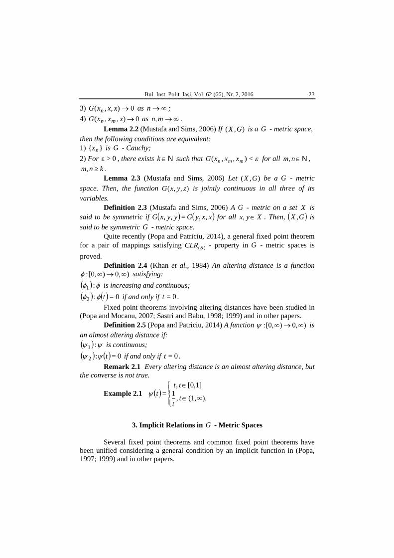
Example 2.1 ( )
∞∈
∈
).(1, ,10,1][ ,
= tt
tttψ
3. Implicit Relations in G - Metric Spaces
Several fixed point theorems and common fixed point theorems have
been unified considering a general condition by an implicit function in (Popa, 1997; 1999) and in other papers.
Valeriu Popa and Alina-Mihaela Patriciu
24
Recently, the method is used in the study of fixed points in metric spaces, symmetric spaces, quasi - metric spaces, b - metric spaces, ultra - metric spaces, reflexive spaces, compact metric spaces, paracompact metric spaces, in two and three metric spaces, for single - valued mappings, hybrid pairs of mappings and set - valued mappings. The method is used in the study of fixed points for mappings satisfying a contractive/extensive condition of integral type, in fuzzy metric spaces, probabilistic metric spaces, intuitionistic metric spaces, partial metric spaces and G - metric spaces.
The study of fixed points for mappings satisfying implicit relations in G - metric spaces is initiated in (Popa and Patriciu, 2012; 2013) and in other papers.
With this method the proofs of some fixed point theorems are more simple. Also, the method allows the study of local and global properties of fixed point structures.
The study of fixed points for pairs of self mappings with common limit range property in metric spaces satisfying implicit relations is initiated in (Imdad and Chauhan, 2013).
The study of fixed points for a pair of self mappings with common limit range property in G - metric spaces is initiated in (Popa and Patriciu, 2014).
In 2008, Ali and Imdad (Ali and Imdad, 2008) introduced a new class of implicit relations.
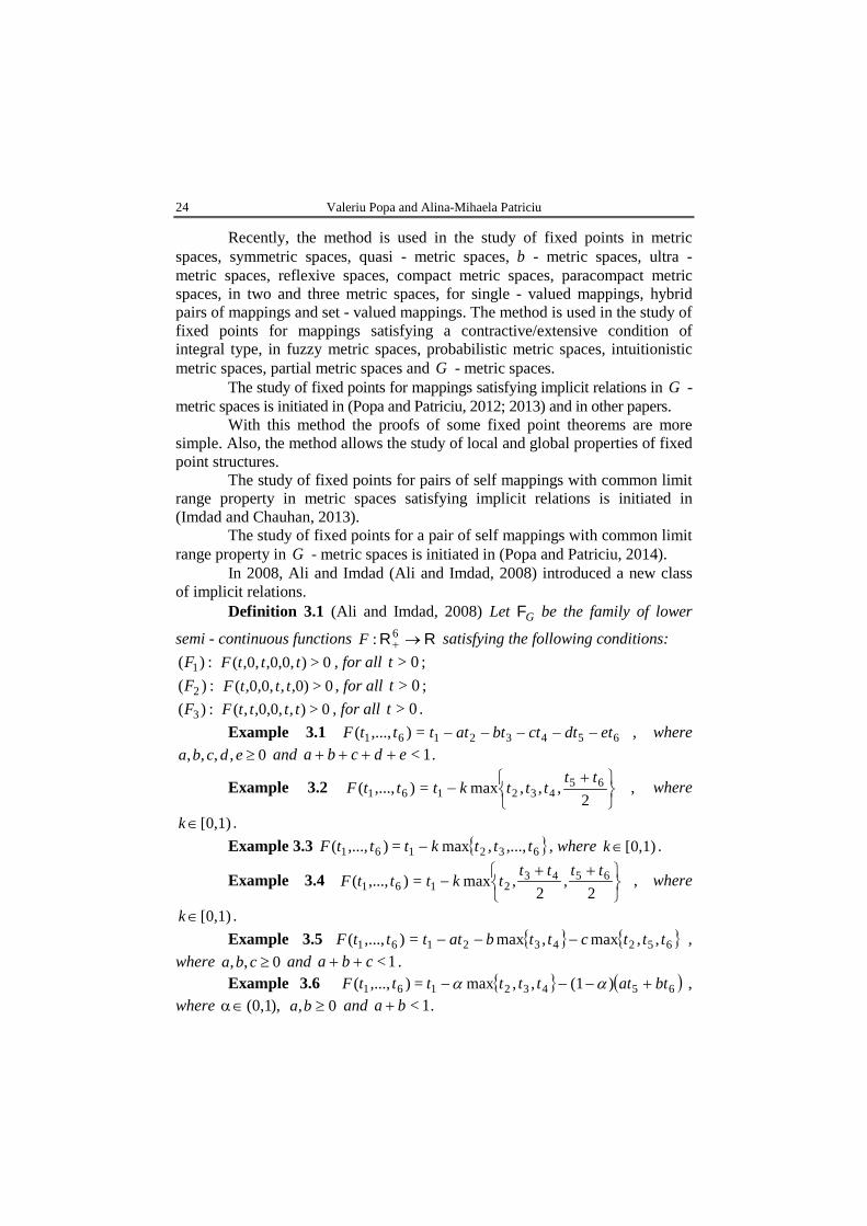
Definition 3.1 (Ali and Imdad, 2008) Let GF be the family of lower
semi - continuous functions RR →+6:F satisfying the following conditions:
:)( 1F 0>),0,0,,0,( tttF , for all 0>t ; :)( 2F 0>,0),,0,0,( tttF , for all 0>t ; :)( 3F 0>),,0,0,,( ttttF , for all 0>t .
Example 3.1 65432161 =),...,( etdtctbtattttF −−−−− , where 0,,,, ≥edcba and 1<edcba ++++ .
Example 3.2
+
−2
,,,max=),...,( 65432161
tttttktttF , where
0,1)[∈k . Example 3.3 { }632161 ,...,,max=),...,( tttktttF − , where 0,1)[∈k .
Example 3.4
++
−2
,2
,max=),...,( 65432161
tttttktttF , where
0,1)[∈k . Example 3.5 { } { }652432161 ,,max,max=),...,( tttcttbattttF −−− ,
where 0,, ≥cba and 1<cba ++ . Example 3.6 { } ( )65432161 )(1,,max=),...,( btatttttttF +−−− αα ,
where ,)0,1(∈α 0, ≥ba and 1<ba + .
Bul. Inst. Polit. Iaşi, Vol. 62 (66), Nr. 2, 2016 25
Example 3.7 ( ) },{min=),...,( 65432161 ttcttbattttF −+−− , where 0>,, cba and 1<cba ++ .
Example 3.8 ( )43
652161 1
=),...,(tt
ttbattttF
+++
−− , where 0, ≥ba and
1<2ba + . Example 3.9 { }65432161 ,,,max=),...,( btatctctcttttF +− , where ,)0,1(∈c 0, ≥ba and 1<cba ++ . Quite recently, the following theorem is proved in (Popa & Patriciu,
2014). Theorem 3.1 (Popa & Patriciu, 2014) Let T and S be self mappings of
a G - metric space ( )GX , such that
0,<))),,((,)),,((,)),,((,)),,((,)),,((,)),,(((
SySxTxGTySxSxGSyTyTyGSxTxTxGSySxSxGTyTxTxGF
ψψψψψψ
for all Xyx ∈, , where F satisfies properties ( ) ( )31 , FF and ψ is an almost altering distance. If T and S satisfy )(SCLR - property, then ( ) ∅≠STC , . Moreover, if T and S are weakly compatible, then T and S have a unique common fixed point.
The purpose of this paper is to prove a general fixed point theorem for two pairs of mappings satisfying common limit range property in G - metric spaces, generalizing the results from (Popa and Patriciu, 2014) and unifying the results from (Giniswamy and Maheshwari, 2014). Also, a new result for a sequence of mappings is obtained.
In the last part of this paper, as applications, some fixed point results for mappings satisfying contractive conditions of integral type, for almost contractive mappings, for ϕ - contractive mappings and ( )ψϕ, - contractive mappings in G - metric spaces are obtained.
4. Main Results
Lemma 4.1 (Abbas and Rhoades, 2009) Let gf , be two weakly compatible self mappings of a nonempty set X . If f and g have a unique point of coincidence gxfxw == for some Xx∈ , then w is the unique common fixed point of f and g .
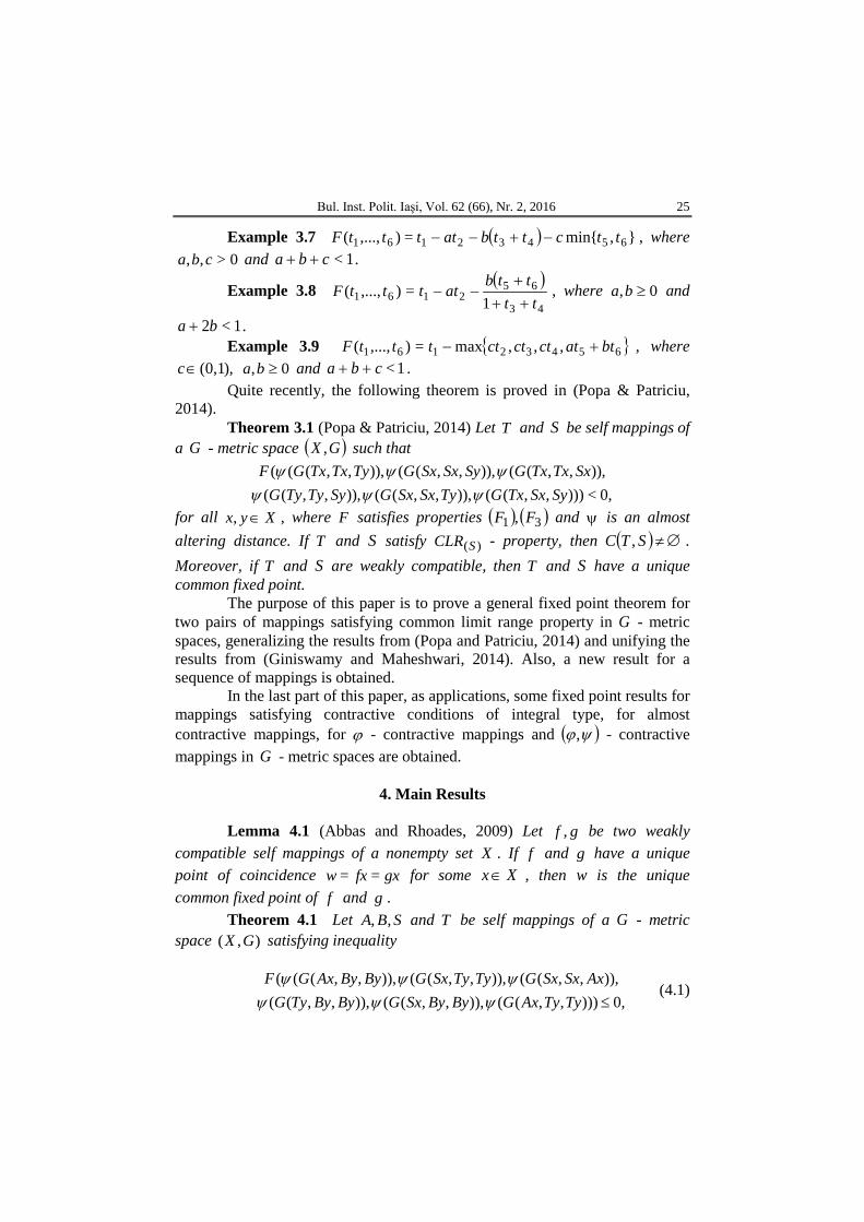
Theorem 4.1 Let SBA ,, and T be self mappings of a G - metric space ),( GX satisfying inequality
0,))),,((,)),,((,)),,((,)),,((,)),,((,)),,(((
≤TyTyAxGByBySxGByByTyGAxSxSxGTyTySxGByByAxGF
ψψψψψψ
(4.1)
Valeriu Popa and Alina-Mihaela Patriciu
26
for all Xyx ∈, , F satisfies property )( 3F and ψ is an almost altering distance.
If there exist Xvu ∈, such that SuAu = and TvBv = , then there exists Xt ∈ such that t is the unique point of coincidence of A and S , as well t is the unique point of coincidence of B and T .
Proof. First we prove that TvSu = . Suppose that TvSu ≠ . By (4.1) we obtain
0,))),,((,)),,((,)),,((,)),,((,)),,((,)),,(((
≤TvTvAuGBvBvSuGBvBvTvGAuSuSuGTvTvSuGBvBvAuGF
ψψψψψψ
0,))),,((,)),,((,0,0,)),,((,)),,((( ≤TvTvSuGTvTvSuGTvTvSuGTvTvSuGF ψψψψa contradiction of )( 3F . Hence, TvSu = , which implies tTvBvAuSu ==== . Suppose that there exists SwAwz == with tz ≠ . Then, by (4.1) we obtain
0,))),,((,)),,((,)),,((,)),,((,)),,((,)),,(((
≤TvTvAwGBvBvSwGBvBvTvGAwSwSwGTvTvSwGBvBvAwGF
ψψψψψψ
0,))),,((,)),,((,0,0,)),,((,)),,((( ≤TvTvSwGTvTvSwGTvTvSwGTvTvSwGF ψψψψa contradiction of )( 3F . Hence, tSuAuBvTvAwSwz ======= and t is the unique point of coincidence of A and S . Similarly, t is the unique point of coincidence of B and T .
Theorem 4.2 Let SBA ,, and T be self mappings of a G - metric space ),( GX satisfying inequality (4.1) for all Xyx ∈, , GF F∈ and ψ is an almost altering distance. If ),( SA and ),( TB satisfy ),( TSCLR - property, then i) ,),( ∅≠SAC ii) .),( ∅≠TBC
Moreover, if ),( SA and ),( TB are weakly compatible, then SBA ,, and T have a unique common fixed point.
Proof. Since ),( SA and ),( TB satisfy ),( TSCLR - property, there exists two sequences }{ nx and }{ ny in X such that
zTyBySxAx nnnnnnnn =lim=lim=lim=lim ∞→∞→∞→∞→ , where )()( XTXSz ∩∈ .
Since )(XTz∈ , there exists Xu∈ such that Tuz = . By (4.1) we have
0.))),,((,)),,((,)),,((,)),,((,)),,((,)),,(((
≤TuTuAxGBuBuSxGBuBuTuGAxSxSxGTuTuSxGBuBuAxGF
nn
nnnnn
ψψψψψψ
Bul. Inst. Polit. Iaşi, Vol. 62 (66), Nr. 2, 2016 27
Letting n tends to infinity we obtain 0,,0))),,((,)),,((,0,0,)),,((( ≤BuBuzGBuBuzGBuBuzGF ψψψ
a contradiction of )( 2F if 0>)),,(( BuBuzGψ . Hence, 0=)),,(( BuBuzGψ , which implies TuBuz == and ∅≠),( TBC .
Since )(XSz∈ , there exists Xv∈ such that Svz = . By (4.1) we obtain
0,))),,((,)),,((,)),,((,)),,((,)),,((,)),,(((
≤TuTuAvGBuBuSvGBuBuTuGAvSvSvGTuTuSvGBuBuAvGF
ψψψψψψ
0,))),,((,0,0,)),,((,0,)),,((( ≤zzAvGzzAvGzzAvGF ψψψ a contradiction of )( 1F if 0>)),,(( zzAvGψ . Hence, 0=)),,(( zzAvGψ , which implies SvAvz == and ∅≠),( SAC .
By Theorem 4.1, z is the unique point of coincidence of ),( SA and ),( TB .
Moreover, if ),( SA and ),( TB are weakly compatible, by Lemma 4.1, z is the unique fixed point of SBA ,, and T .
If tt =)(ψ , then by Theorem 4.2 we obtain Theorem 4.3 Let SBA ,, and T be self mappings of a G - metric
space ),( GX satisfying the inequality
0,)),,(),,,(),,,(),,,(),,,(),,,((≤TyTyAxGByBySxGByByTyG
AxSxSxGTyTySxGByByAxGF (4.2)
for all Xyx ∈, , GF F∈ .
If ),( SA and ),( TB satisfy ),( TSCLR - property, then i) ,),( ∅≠SAC ii) .),( ∅≠TBC
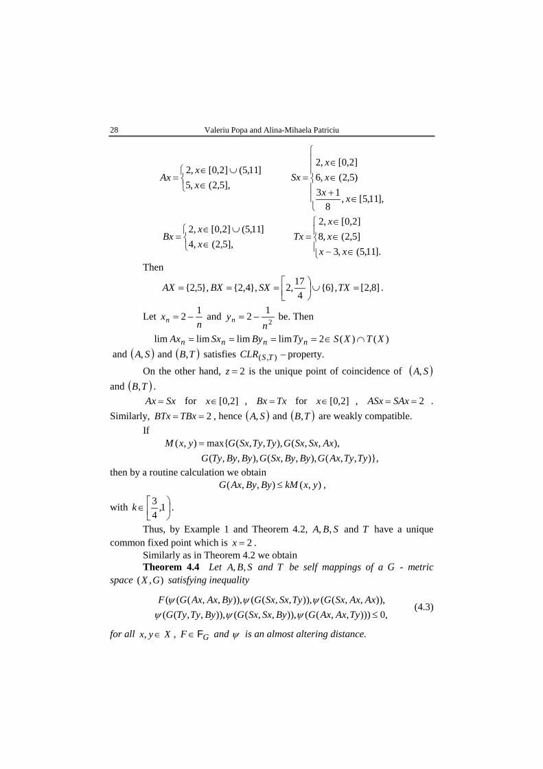
Moreover, if ),( SA and ),( TB are weakly compatible, then SBA ,, and T have a unique common fixed point. Example 4.1 Let ]11,0[=X and let +→R3: XG be the G – metric defined as follows
|}||,||,max{|),,( zxzyyxzyxG −−−= for all Xzyx ∈,, . Then ),( GX is a G – metric space. Define the self mappings SBA ,, and T
Valeriu Popa and Alina-Mihaela Patriciu
28
∈∪∈
=],5,2(,5
]11,5(]2,0[,2xx
Ax
∈+∈∈
=
],11,5[,8
13)5,2(,6]2,0[,2
xxxx
Sx
∈∪∈
=],5,2(,4
]11,5(]2,0[,2xx
Bx
∈−∈∈
=].11,5(,3
]5,2(,8]2,0[,2
xxxx
Tx
Then
]8,2[},6{4
17,2},4,2{},5,2{ =∪
=== TXSXBXAX .
Let n
xn12 −= and 2
12n
yn −= be. Then
)()(2limlimlimlim XTXSTyBySxAx nnnn ∩∈==== and ( )SA, and ( )TB, satisfies −),( TSCLR property.
On the other hand, 2=z is the unique point of coincidence of ( )SA, and ( )TB, . SxAx = for ]2,0[∈x , TxBx = for ]2,0[∈x , 2== SAxASx . Similarly, 2==TBxBTx , hence ( )SA, and ( )TB, are weakly compatible. If
)},,,(),,,(),,,(),,,(),,,(max{),(
TyTyAxGByBySxGByByTyGAxSxSxGTyTySxGyxM =
then by a routine calculation we obtain ),(),,( yxkMByByAxG ≤ ,
with
∈ 1,
43k .
Thus, by Example 1 and Theorem 4.2, SBA ,, and T have a unique common fixed point which is 2=x .
Similarly as in Theorem 4.2 we obtain Theorem 4.4 Let SBA ,, and T be self mappings of a G - metric
space ),( GX satisfying inequality
0,))),,((,)),,((,)),,((,)),,((,)),,((,)),,(((
≤TyAxAxGBySxSxGByTyTyGAxAxSxGTySxSxGByAxAxGF
ψψψψψψ
(4.3)
for all Xyx ∈, , GF F∈ and ψ is an almost altering distance.
Bul. Inst. Polit. Iaşi, Vol. 62 (66), Nr. 2, 2016 29
If ),( SA and ),( TB satisfy ),( TSCLR - property, then i) ,),( ∅≠SAC ii) .),( ∅≠TBC
Moreover, if ),( SA and ),( TB are weakly compatible, then SBA ,, and T have a unique common fixed point.
Theorem 4.5 Let ),( GX be a G - metric space and SBA ,, and T be self mappings of X satisfying the inequality
),,,(),,(),,(),,(),,(),,(TyTyAxeGByBySxdGByByTycG
AxSxSxbGTyTySxaGByByAxG+++
++≤
(4.4)
for all Xyx ∈, , 0,,,, ≥edcba and 1<edcba ++++ . If ),( SA and ),( TB satisfy ),( TSCLR - property, then
i) ,),( ∅≠SAC ii) .),( ∅≠TBC
Moreover, if ),( SA and ),( TB are weakly compatible, then SBA ,, and T have a unique common fixed point.
Corollary 4.1 (Theorem 2.5 (Giniswamy and Maheshwari, 2014)) Let ),( GX be a G - metric space and SBA ,, and T be self mappings of X such
that: 1) ),( SA and ),( TB satisfy ),( TSCLR - property;
2) )],,,(),,([),,(
),,(),,(),,(BzBySxGTzTyAxGtBzBzTyrG
AxSxSxqGTyTySxpGBzByAxG+++
++≤
(4.5)
for all Xzyx ∈,, , where 0,,, ≥trqp and 1<2trqp +++ . Then ),( SA and ),( TB have a unique point of coincidence in X . Moreover, if ),( SA and ),( TB are weakly compatible, then SBA ,,
and T have a unique common fixed point. Proof. Let zy = , then by (4.5) we obtain a particular case of (4.4) and
the proof follows from Theorem 4.5. Theorem 4.6 Let ),( GX be a G - metric space and SBA ,, and T be
self mappings of X satisfying the inequality:
},2
),,(),,(),,,(
),,,(),,,({max),,(TyTyAxGByBySxGByByTyG
AxSxSxGTyTySxGkByByAxG+
≤
(4.6)
for all Xyx ∈, and 0,1)[∈k . If ),( SA and ),( TB satisfy ),( TSCLR - property, then
i) ,),( ∅≠SAC ii) .),( ∅≠TBC
Valeriu Popa and Alina-Mihaela Patriciu
30
Moreover, if ),( SA and ),( TB are weakly compatible, then SBA ,, and T have a unique common fixed point.
Proof. The proof follows from Theorem 4.3 and Example 3.2. Corollary 4.2 (Theorem 2.6 (Giniswamy and Maheshwari, 2014)) Let
),( GX be a G - metric space and SBA ,, and T be self mappings of X such that: 1) ),( SA and ),( TB satisfy ),( TSCLR - property; 2) ),,(),,( zyxhuBzByAxG ≤ , where )0,1(∈h , Xzyx ∈,, and
}.2
),,(),,(,),,(,),,(,),,({),,( BzBySxGTzTyAxGByByTyGTyTySxGSxSxAxGzyxu +∈
Then ),( SA and ),( TB have a unique point of coincidence in X . Moreover, if ),( SA and ),( TB are weakly compatible, then SBA ,,
and T have a unique common fixed point. Proof. Let zy = , then by (2) we obtain
},2
),,(),,(,),,(
,),,(,),,({max),,(TyTyAxGByBySxGByByTyG
AxSxSxGTyTySxGhByByAxG+
≤
which is inequality (4.6) and the proof of Corollary 4.2 follows from Theorem 4.6.
For a function XXf →: we denote
}.=:{=)( fxxXxfFix ∈
Theorem 4.7 Let SBA ,, and T be self mappings of a G - metric space ),( GX . If the inequality (4.1) holds for all Xyx ∈, , GF F∈ and ψ is an almost altering distance, then
[ ] [ ] .)()()(=)()()( BFixTFixSFixAFixTFixSFix ∩∩∩∩ Proof. Let [ ] )()()( AFixTFixSFixx ∩∩∈ . Then by (4.1) we have
0,))),,((,)),,((,)),,((,)),,((,)),,((,)),,(((
≤TxTxAxGBxBxSxGBxBxTxGAxSxSxGTxTxSxGBxBxAxGF
ψψψψψψ
0,,0))),,((,)),,((,0,0,)),,((( ≤BxBxxGBxBxxGBxBxxGF ψψψ a contradiction of )( 2F if 0>)),,(( BxBxxGψ . Hence, 0=)),,(( BxBxxGψ which implies Bxx = and )(BFixx∈ .
Hence [ ] [ ] .)()()()()()( BFixTFixSFixAFixTFixSFix ∩∩⊂∩∩
Similarly, by (4.1) and )( 1F we obtain [ ] [ ] .)()()()()()( AFixTFixSFixBFixTFixSFix ∩∩⊂∩∩
Theorems 4.2 and 4.7 imply the following one.
Bul. Inst. Polit. Iaşi, Vol. 62 (66), Nr. 2, 2016 31
Theorem 4.8 Let TS , and ∗∈NiiA }{ be self mappings of a G - metric
space ),( GX satisfying the inequality
0,))),,((,)),,((,)),,((,)),,((,)),,((,)),,(((
1111
11
≤++++
++
TyTyxAGyAyASxGyAyATyGxASxSxGTyTySxGyAyAxAGF
iiiii
iiii
ψψψψψψ
(4.7)
for all Xyx ∈, , GF F∈ , ψ is an almost altering distance and ∗∈Ni . If ),( 1 SA and ),( 2 TA satisfy ),( TSCLR - property and ),(,),( 21 TASA
are weakly compatible, then TS , and ∗∈NiiA }{ have a unique common fixed
point. If ( ) tt =ψ , from Theorem 4.8 we obtain Theorem 4.9 Let TS , and ∗∈NiiA }{ be self mappings of a G - metric
space ),( GX satisfying the inequality
0,)),,(),,,(),,,(),,,(),,,(),,,((
1111
11
≤++++
++
TyTyxAGyAyASxGyAyATyGxASxSxGTyTySxGyAyAxAGF
iiiii
iiii (4.8)
for all Xyx ∈, , GF F∈ and ∗∈Ni . If ),( 1 SA and ),( 2 TA satisfy ),( TSCLR - property and ),(,),( 21 TASA
are weakly compatible, then TS , and ∗∈NiiA }{ have a unique common fixed
point. Remark 4.1 We obtain similar results from Theorem 4.4.
5. Applications
5.1. Fixed Points for Mappings Satisfying Contractive Conditions of Integral Type
In (Branciari, 2002), Branciari established the following theorem which opened the way to the study of fixed points for mappings satisfying contractive conditions of integral type. Theorem 5.1 (Branciari, 2002) Let ),( dX be a complete metric space,
)1,0(∈c and XXf →: such that for all Xyx ∈,
∫∫ ≤),(
0
),(
0)()(
yxdfyfxddtthcdtth ,
whenever ),0[),0[: ∞→∞h is a Lebesgue measurable mapping which is summable (i.e., with finite integral) on each compact subset of ),0[ ∞ such that
Valeriu Popa and Alina-Mihaela Patriciu
32
0)(0
>∫ε
dtth for each 0>ε . Then, f has an unique fixed point Xz∈ such that
for all Xx∈ , xfz nn ∞→
= lim .
Theorem 5.1 has been extended to a pair of compatible mappings in (Kumar et al., 2007). Theorem 5.2 (Kumar et al., 2007) Let gf , be compatible mappings of a complete metric space with g – continuous satisfying the following conditions: 1) )()( XgXf ⊂ ,
2) ∫≤∫),(
0
),(
0)()(
yxdgyfxddtthcdtth ,
for some )1,0(∈c , whenever Xyx ∈, and )(th as in Theorem 5.1. Then, f and g have a unique common fixed point. Some fixed point results for mappings satisfying contractive conditions of integral type are proved in (Popa and Mocanu, 2007; 2009) and in other papers.
Lemma 5.1 Let )0,)[0,: ∞→∞h as in Theorem 5.1. Then
dxxht t )(=)( 0∫ψ is an almost altering distance. Proof. The proof follows from Lemma 2.5 (Popa and Mocanu, 2009). Theorem 5.3 Let SBA ,, and T be self mappings of a G - metric
space ),( GX such that
0,))(,)(,)(
,)(,)(,)((),,(
0),,(
0),,(
0
),,(0
),,(0
),,(0
≤∫∫∫
∫∫∫dtthdtthdtth
dtthdtthdtthFTyTyAxGByBySxGByByTyG
AxSxSxGTyTySxGByByAxG
(5.1)
for all Xyx ∈, , where GF F∈ and )(th as in Theorem 5.1. If ),( SA and ),( TB satisfy ),( TSCLR - property, then
i) ,),( ∅≠SAC ii) .),( ∅≠TBC
Moreover, if ),( SA and ),( TB are weakly compatible, then SBA ,, and T have a unique common fixed point.
Proof. By Lemma 5.1, dxxht t )(=)( 0∫ψ is an almost altering distance. By (5.1) we have
0.))),,(()),,,(()),,,(()),,,(()),,,(()),,,(((≤TyTyAxGByBySxGByByTyG
AxSxSxGTyTySxGByByAxGFψψψ
ψψψ
Bul. Inst. Polit. Iaşi, Vol. 62 (66), Nr. 2, 2016 33
Hence the conditions of Theorem 4.2 are satisfied and the conclusions of Theorem 5.3 follows.
Similarly, from Theorem 4.4 we obtain Theorem 5.4 Let SBA ,, and T be self mappings of a G - metric
space ),( GX such that
0,))(,)(,)(
,)(,)(,)((),,(
0),,(
0),,(
0
),,(0
),,(0
),,(0
≤∫∫∫
∫∫∫dtthdtthdtth
dtthdtthdtthFTyAxAxGBySxSxGByTyTyG
AxSxSxGBySxSxGByAxAxG
(5.2)
for all Xyx ∈, , where GF F∈ and )(th as in Theorem 5.1. If ),( SA and ),( TB satisfy ),( TSCLR - property, then
i) ,),( ∅≠SAC ii) .),( ∅≠TBC
Moreover, if ),( SA and ),( TB are weakly compatible, then SBA ,, and T have a unique common fixed point.
From Theorem 5.4 and Example 3.2 we obtain Theorem 5.5 Let ),( GX be a G - metric space and SBA ,, and T be
self mappings of X satisfying
},2
)()(,)(
,)(,)({max)(),,(
0),,(
0),,(0
),,(0
),,(0
),,(0
dtthdtthdtth
dtthdtthkdtthTyAxAxGBySxSxG
ByTyTyG
AxSxSxGTySxSxGByAxAxG
∫∫∫
∫∫∫+
≤
for all Xyx ∈, , 0,1)[∈k and )(th as in Theorem 5.1. If ),( SA and ),( TB satisfy ),( TSCLR - property, then
i) ,),( ∅≠SAC ii) .),( ∅≠TBC
Moreover, if ),( SA and ),( TB are weakly compatible, then SBA ,, and T have a unique common fixed point.
Remark 5.1 If 1=)(th , from Theorem 5.5 we obtain Theorem 4.6. From Theorems 5.3, 5.4 and Examples 3.1 – 3.9 we obtain new
particular results.
5.2. Fixed Points for Almost Contractive Mappings in G - Metric Spaces
Definition 5.1 Let ),( dX be a metric space. A mapping XXT →: is
called weak contractive (Berinde, 2003; 2004) or almost contractive (Berinde, 2010) if there exist )0,1(∈δ and some 0≥L such that
.,),(),(),( XyxallforTxyLdyxdTyTxd ∈+δ≤
Valeriu Popa and Alina-Mihaela Patriciu
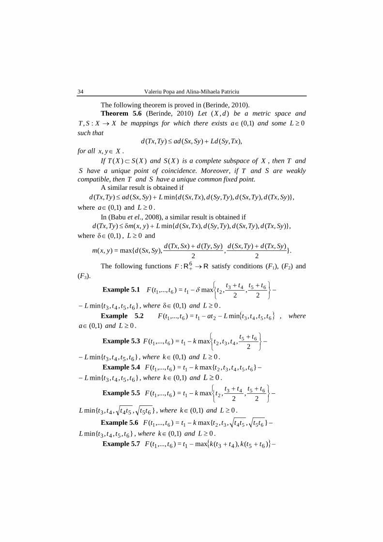
34
The following theorem is proved in (Berinde, 2010). Theorem 5.6 (Berinde, 2010) Let ),( dX be a metric space and
XXST →:, be mappings for which there exists )0,1(∈a and some 0≥L such that
,),(),(),( TxSyLdSySxadTyTxd +≤ for all Xyx ∈, .
If )()( XSXT ⊂ and )(XS is a complete subspace of X , then T and S have a unique point of coincidence. Moreover, if T and S are weakly compatible, then T and S have a unique common fixed point.
A similar result is obtained if },),(,),(,),(,),({min),(),( SyTxdTySxdTySydTxSxdLSySxadTyTxd +≤
where )0,1(∈a and 0≥L . In (Babu et el., 2008), a similar result is obtained if
},),(,),(,),(,),({min),(),( SyTxdTySxdTySydTxSxdLyxmTyTxd +δ≤ where )0,1(∈δ , 0≥L and
}.2
),(),(,2
),(),(,),({max=),( SyTxdTySxdSyTydSxTxdSySxdyxm ++
The following functions RR →+6:F satisfy conditions (F1), (F2) and
(F3).
Example 5.1 −
++
−2
,2
,max=),...,( 65432161
ttttttttF δ
},,,min{ 6543 ttttL− , where )0,1(∈δ and 0≥L .
Example 5.2 { }65432161 ,,,min=),...,( ttttLattttF −− , where )0,1(∈a and 0≥L .
Example 5.3 −
+
−2
,,,max=),...,( 65432161
tttttktttF
},,,min{ 6543 ttttL− , where )0,1(∈k and 0≥L .
Example 5.4 −− },,,,max{=),...,( 65432161 tttttktttF },,,min{ 6543 ttttL− , where )0,1(∈k and 0≥L .
Example 5.5 −
++
−2
,2
,max=),...,( 65432161
tttttktttF
},,,min{ 655443 ttttttL , where )0,1(∈k and 0≥L .
Example 5.6 −− },,,max{=),...,( 655432161 ttttttktttF },,,min{ 6543 ttttL , where )0,1(∈k and 0≥L .
Example 5.7 { }−++− )(,)(max=),...,( 6543161 ttkttktttF
Bul. Inst. Polit. Iaşi, Vol. 62 (66), Nr. 2, 2016 35
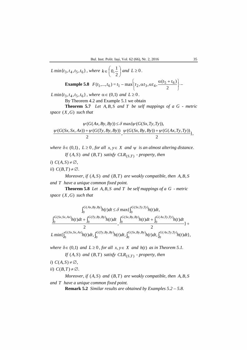
},,,min{ 6543 ttttL , where
∈
210,k and 0≥L .
Example 5.8 −
+α
αα−2
)(,,,max=),...,( 65
432161tt
ttttttF
},,,min{ 6543 ttttL , where )0,1(∈α and 0≥L . By Theorem 4.2 and Example 5.1 we obtain Theorem 5.7 Let SBA ,, and T be self mappings of a G - metric
space ),( GX such that
},2
)),,(()),,((,2
)),,(()),,(()),,,(({max)),,((
TyTyAxGByBySxGByByTyGAxSxSxGTyTySxGByByAxGψψψψ
ψδψ++
≤
where )0,1(∈δ , 0≥L , for all Xyx ∈, and ψ is an almost altering distance.
If ),( SA and ),( TB satisfy ),( TSCLR - property, then
i) ,),( ∅≠SAC ii) .),( ∅≠TBC
Moreover, if ),( SA and ),( TB are weakly compatible, then SBA ,, and T have a unique common fixed point.
Theorem 5.8 Let SBA ,, and T be self mappings of a G - metric space ),( GX such that
},)(,)(,)(,)({min
}2
)()(,
2
)()(
,)({max)(
),,(0
),,(0
),,(0
),,(0
),,(0
),,(0
),,(0
),,(0
),,(0
),,(0
dtthdtthdtthdtthL
dtthdtthdtthdtth
dtthdtth
TyTyAxGByBySxGByByTyGAxSxSxG
TyTyAxGByBySxGByByTyGAxSxSxG
TyTySxGByByAxG
∫∫∫∫
∫∫∫∫
∫∫
+++
≤ δ
where )0,1(∈δ and 0≥L , for all Xyx ∈, and )(th as in Theorem 5.1.
If ),( SA and ),( TB satisfy ),( TSCLR - property, then
i) ,),( ∅≠SAC ii) .),( ∅≠TBC
Moreover, if ),( SA and ),( TB are weakly compatible, then SBA ,, and T have a unique common fixed point.
Remark 5.2 Similar results are obtained by Examples 5.2 – 5.8.
Valeriu Popa and Alina-Mihaela Patriciu
36
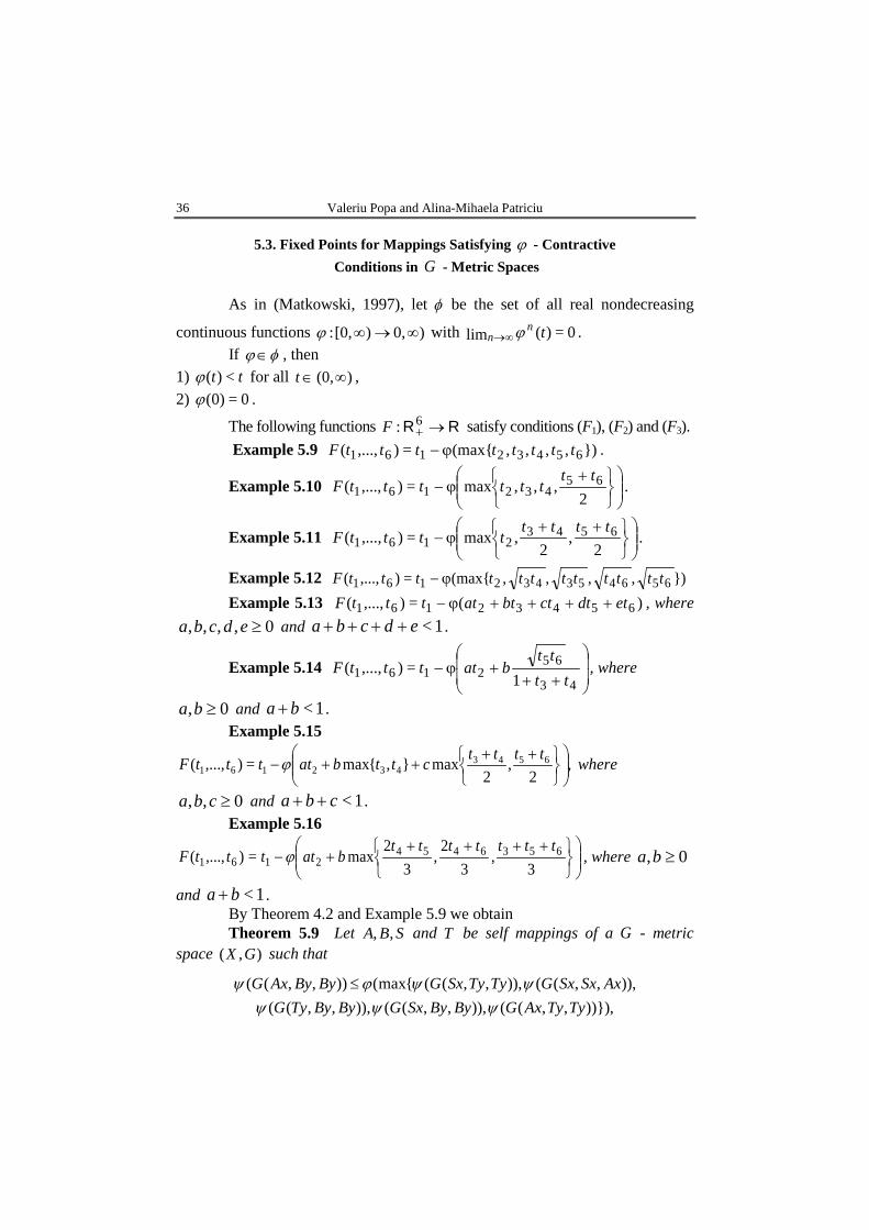
5.3. Fixed Points for Mappings Satisfying ϕ - Contractive Conditions in G - Metric Spaces
As in (Matkowski, 1997), let φ be the set of all real nondecreasing
continuous functions )0,)[0,: ∞→∞ϕ with 0=)(lim tnn ϕ∞→ .
If φϕ∈ , then 1) tt <)(ϕ for all )(0,∞∈t , 2) 0=)0(ϕ .
The following functions RR →+6:F satisfy conditions (F1), (F2) and (F3).
Example 5.9 }),,,,(max{=),...,( 65432161 ttttttttF ϕ− .
Example 5.10
+
ϕ−2
,,,max=),...,( 65432161
ttttttttF .
Example 5.11
++
ϕ−2
,2
,max=),...,( 65432161
ttttttttF .
Example 5.12 }),,,,(max{=),...,( 656453432161 ttttttttttttF ϕ− Example 5.13 )(=),...,( 65432161 etdtctbtattttF ++++ϕ− , where
0,,,, ≥edcba and 1<edcba ++++ .
Example 5.14
+++ϕ−
43
652161 1
=),...,(tt
ttbattttF , where
0, ≥ba and 1<ba + . Example 5.15
,2
,2
max},{max=),...,( 6543432161
++
++−ttttcttbattttF ϕ where
0,, ≥cba and 1<cba ++ . Example 5.16
++++
+−3
,3
2,
32
max=),...,( 65364542161
tttttttbattttF ϕ , where 0, ≥ba
and 1<ba + . By Theorem 4.2 and Example 5.9 we obtain Theorem 5.9 Let SBA ,, and T be self mappings of a G - metric
space ),( GX such that
,)})),,(()),,,(()),,,(()),,,(()),,,(({max()),,((
TyTyAxGByBySxGByByTyGAxSxSxGTyTySxGByByAxG
ψψψψψϕψ ≤
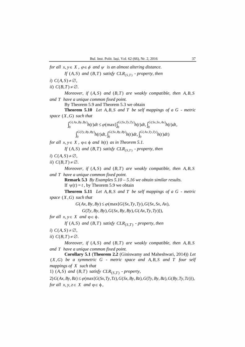
Bul. Inst. Polit. Iaşi, Vol. 62 (66), Nr. 2, 2016 37
for all Xyx ∈, , φϕ∈ and ψ is an almost altering distance. If ),( SA and ),( TB satisfy ),( TSCLR - property, then
i) ,),( ∅≠SAC ii) .),( ∅≠TBC
Moreover, if ),( SA and ),( TB are weakly compatible, then SBA ,, and T have a unique common fixed point.
By Theorem 5.9 and Theorem 5.3 we obtain Theorem 5.10 Let SBA ,, and T be self mappings of a G - metric
space ),( GX such that
))(,)(,)(
,)(,)({max()(),,(
0),,(
0),,(
0
),,(0
),,(0
),,(0
dtthdtthdtth
dtthdtthdtthTyTyAxGByBySxGByByTyG
AxSxSxGTyTySxGByByAxG
∫∫∫
∫∫∫ ≤ϕ
for all Xyx ∈, , φ∈ϕ and )(th as in Theorem 5.1. If ),( SA and ),( TB satisfy ),( TSCLR - property, then
i) ,),( ∅≠SAC ii) .),( ∅≠TBC
Moreover, if ),( SA and ),( TB are weakly compatible, then SBA ,, and T have a unique common fixed point.
Remark 5.3 By Examples 5.10 – 5.16 we obtain similar results. If tt =)(ψ , by Theorem 5.9 we obtain Theorem 5.11 Let SBA ,, and T be self mappings of a G - metric
space ),( GX such that
),}),,(),,,(),,,(),,,(),,,({max(),,(
TyTyAxGByBySxGByByTyGAxSxSxGTyTySxGByByAxG ϕ≤
for all Xyx ∈, and φ∈ϕ . If ),( SA and ),( TB satisfy ),( TSCLR - property, then
i) ,),( ∅≠SAC ii) .),( ∅≠TBC
Moreover, if ),( SA and ),( TB are weakly compatible, then SBA ,, and T have a unique common fixed point.
Corollary 5.1 (Theorem 2.2 (Giniswamy and Maheshwari, 2014)) Let ),( GX be a symmetric G - metric space and SBA ,, and T four self
mappings of X such that 1) ),( SA and ),( TB satisfy ),( TSCLR - property, 2) }),),,(),,,(,),,(,),,({max(),,( TzTyByGBzByTyGBzBySxGTzTySxGBzByAxG ϕ≤ for all Xzyx ∈,, and φ∈ϕ ,
Valeriu Popa and Alina-Mihaela Patriciu
38
3) ),( SA and ),( TB are weakly compatible. Then SBA ,, and T have a unique common fixed point. Proof. If zy = , by 2) we have
}).),,(),,,(,),,(,),,({max(),,( TyTyByGByByTyGByBySxGTyTySxGByByAxG ϕ≤
Since ),( GX is symmetric and ϕ is non decreasing, then
,})),,(,),,(,),,(,),,(,),,({max(})),,(,),,(,),,({max(),,(
TyTyAxGByBySxGByByTyGAxSxSxGTyTySxGByTyTyGByBySxGTyTySxGByByAxG
ϕϕ
≤≤
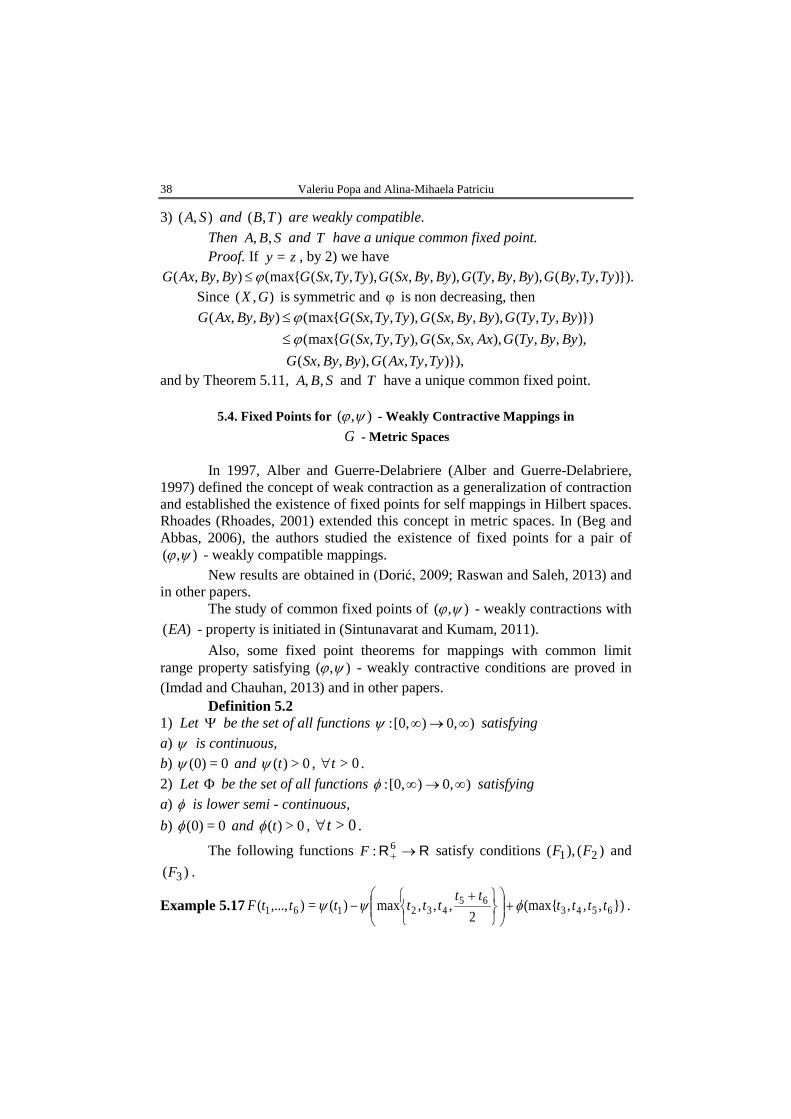
and by Theorem 5.11, SBA ,, and T have a unique common fixed point.
5.4. Fixed Points for ),( ψϕ - Weakly Contractive Mappings in G - Metric Spaces
In 1997, Alber and Guerre-Delabriere (Alber and Guerre-Delabriere,
1997) defined the concept of weak contraction as a generalization of contraction and established the existence of fixed points for self mappings in Hilbert spaces. Rhoades (Rhoades, 2001) extended this concept in metric spaces. In (Beg and Abbas, 2006), the authors studied the existence of fixed points for a pair of
),( ψϕ - weakly compatible mappings. New results are obtained in (Dorić, 2009; Raswan and Saleh, 2013) and
in other papers. The study of common fixed points of ),( ψϕ - weakly contractions with
)(EA - property is initiated in (Sintunavarat and Kumam, 2011). Also, some fixed point theorems for mappings with common limit
range property satisfying ),( ψϕ - weakly contractive conditions are proved in (Imdad and Chauhan, 2013) and in other papers.
Definition 5.2 1) Let Ψ be the set of all functions )0,)[0,: ∞→∞ψ satisfying a) ψ is continuous, b) 0=)0(ψ and 0>)(tψ , 0>t∀ . 2) Let Φ be the set of all functions )0,)[0,: ∞→∞φ satisfying a) φ is lower semi - continuous, b) 0=)0(φ and 0>)(tφ , 0>t∀ .
The following functions RR →+6:F satisfy conditions )(,)( 21 FF and
)( 3F .
Example 5.17 }),,,(max{2
,,,max)(=),...,( 654365
432161 tttttt
ttttttF φψψ +
+
− .
Bul. Inst. Polit. Iaşi, Vol. 62 (66), Nr. 2, 2016 39
Example 5.18
+
φ+ψ−ψ2
,,,max}),,,,(max{)(=),...,( 6543265432161
tttttttttttttF .
Example 5.19
}),,,,(max{2
,2
,max)(=),...,( 654326543
2161 ttttttttt
ttttF φ+
++
ψ−ψ .
Example 5.20
+
φ+
++
ψ−ψ2
,,,max2
,2
,max)(=),...,( 65432
65432161
ttttt
ttttttttF
Example 5.21
}),,(max{2
,,,max)(=),...,( 65526365
432161 tttttttt
ttttttF φ+
+
ψ−ψ
Example 5.22 }),,,,(max{}),,(max{)(=),...,( 65432645263161 ttttttttttttttF φ+ψ−ψ
Example 5.23
}),,,,(max{1
)(=),...,( 65432326443
625463161 ttttt
tttttt
tttttttttF φ+
+++
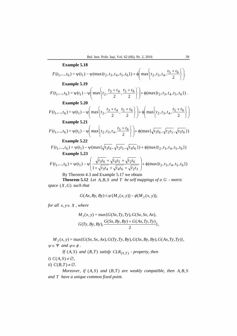
++ψ−ψ
By Theorem 4.3 and Example 5.17 we obtain Theorem 5.12 Let SBA ,, and T be self mappings of a G - metric
space ),( GX such that
,)),(()),((),,( 21 yxMyxMByByAxG φψ −≤ for all Xyx ∈, , where
},2
),,(),,(,),,(
,),,(,),,({max=),(1
TyTyAxGByBySxGByByTyG
AxSxSxGTyTySxGyxM+
},),,(,),,(,),,(,),,({max=),(2 TyTyAxGByBySxGByTyTyGAxSxSxGyxM Ψ∈ψ and φϕ∈ .
If ),( SA and ),( TB satisfy ),( TSCLR - property, then i) ,),( ∅≠SAC ii) .),( ∅≠TBC
Moreover, if ),( SA and ),( TB are weakly compatible, then SBA ,, and T have a unique common fixed point.
Valeriu Popa and Alina-Mihaela Patriciu
40
REFERENCES
Aamri M., El - Moutawakil D., Some New Common Fixed Point Theorems Under Strict
Contractive Conditions, J. Math. Anal. Appl., 270, 181-188 (2002). Abbas M., Rhoades B.E., Common Fixed Point Results for Noncommuting Mappings
Without Continuity in Generalized Metric Spaces, Appl. Math. Comput., 215, 262-269 (2009).
Alber Ya. I., Guerre - Delabriere S., Principle of Weakly Contractive Maps in Hilbert Spaces, New Results in Operator Theory and its Applications, Adv. Appl. Math. (Ed. by Y. Gahbery and Yu. Lybrch), Birkhauser Verlag Basel, 98, 7-22 (1997).
Ali J., Imdad M., An Implicit Function Implies Several Contractive Conditions, Sarajevo J. Math., 17, 4, 269-285 (2008).
Babu G.V.R., Sandhya M., Kameswari M.V.R., A Note on Fixed Point Theorem of Berinde Weak Contraction, Carpathian J. Math., 24, 1, 8-12 (2008).
Beg I., Abbas M., Coincidence Point and Invariant Approximation for Mappings Satisfying Generalized Weak Contractive Condition, Fixed Point Theory Appl., 2006, Article ID 74503, 7 pages (2006).
Berinde V., On the Approximations of Fixed Point of Weak Contractive Mappings, Carpathian J. Math., 19, 1, 87-92 (2003).
Berinde V., Approximating Fixed Points of Weak Contractions Using the Picard Iteration, Nonlinear Anal. Forum, 9, 1, 43-53 (2004).
Berinde V., Approximating Common Fixed Points of Noncommuting Almost Contractions in Metric Spaces, Fixed Point Theory, 11, 10-19 (2010).
Branciari A., A Fixed Point Theorem for Mappings Satisfying a General Contractive Condition of Integral Type, Int. J. Math. Math. Sci., 29, 2, 531-536 (2002).
Dhage B.C., Generalized Metric Spaces and Mappings with Fixed Point, Bull. Calcutta Math. Soc. 84, 4, 329-336 (1992).
Dhage B.C., Generalized Metric Spaces and Topological Structures I, An. Ştiinţ. Univ. Al. I. Cuza, Iaşi, Mat., 46, 1, 3-24 (2000).
Dorić D., Common Fixed Points for Generalized ),( ψϕ - Weak Contractions, Appl. Math. Lett., 22, 1986-2000 (2009).
Giniswamy, Maheshwari P.G., Some Common Fixed Point Theorems on G - Metric Spaces, Gen. Math. Notes, 21, 2, 114-124 (2014).
Imdad M., Pant M., Chauhan B.C., Fixed Point Theorems in Menger Spaces Using ),( TSCLR – Property and Applications, J. Nonlinear Analysis Optim., 312, 2,
225-237 (2012). Imdad M., Chauhan S., Kadelburg Z., Fixed Point Theorems for Mappings with
Common Limit Range Property Satisfying Generalized ),( ϕψ – Weak Contractive, Math. Sci., 7, 16, doi: 10.1186/2251 – 7 – 16 (2013).
Imdad M., Chauhan S., Employing Common Limit Range Property to Prove Unified Metrical Common Fixed Point Theorems, Int. J. Anal., Vol. 2013, Article ID 763261, 10 pages (2013).
Jungck G., Compatible Mappings and Common Fixed Points, Int. J. Math. Math. Sci., 9, 771-779 (1980).
Bul. Inst. Polit. Iaşi, Vol. 62 (66), Nr. 2, 2016 41
Jungck G., Common Fixed Points for Noncontinuous Nonself Maps on Nonnumeric Spaces, Far East J. Math. Sci., 4, 195–215 (1996).
Karapinar E., Patel D.K., Imdad M., Gopal D., Some Non – Unique Common Fixed Point Theorems in Symmetric Spaces Throughout ),( TSCLR – Property, Int. J. Math. Math. Sci., 2013, Article ID 753965, 8 pages.
Khan M.S., Swaleh M., Sessa S., Fixed Point Theorems by Altering Distances Between Points, Bull. Aust. Math. Soc., 30, 1-9 (1984).
Kumar S., Chugh R., Kumar R., Fixed Point Theorems for Compatible Mappings Satisfying a Contractive Condition of Integral Type, Soochow J. Math., 33, 2, 181-185 (2007).
Liu Y., Wu J., Li Z., Common Fixed Points of Single - Valued and Multivalued Maps, Int. J. Math. Math. Sci., 19, 3045-3055 (2005).
Matkowski J., Fixed Point Theorems with a Contractive Iterate at a Point, Proc. Amer. Math. Soc., 62, 2, 344-348 (1997).
Mustafa Z., Sims B., Some Remarks Concerning D - Metric Spaces, Proc. Conf. Fixed Point Theory Appl., Valencia (Spain), 2003, 189-198.
Mustafa Z., Sims B., A New Approach to Generalized Metric Spaces, J. Nonlinear Convex Anal., 7, 289-297 (2006).
Mustafa Z., Obiedat H., Awawdeh F., Some Fixed Point Theorems for Mappings in G - Complete Metric Spaces, Fixed Point Theory Appl., 2008, Article ID 189870.
Mustafa Z., Sims B., Fixed Point Theorems for Contractive Mappings in Complete G - Metric Spaces, Fixed Point Theory Appl. 2009, Article ID 917175.
Pant R.P., R – Weak Commutativity and Common Fixed Points for Noncompatible Maps, Ganita, 99, 19-26 (1998).
Pant R.P., R – Weak Commutativity and Common Fixed Points for Noncompatible Maps, Soochow J. Math., 25, 37-42 (1999).
Pant R.P., Common Fixed Points of Noncommuting Mappings, J. Math. Anal. Appl., 188, 436-440 (1994).
Pathak H.K., Rodriguez – López R., Verma R.K., A Common Fixed Point Theorem of Integral Type Using Implicit Relations, Nonlinear Funct. Anal. Appl., 15, 1, 1-12 (2010).
Popa V., Some Fixed Point Theorems for Implicit Contractive Mappings, Stud. Cercet. Ştiinţ. Ser. Mat., Univ. Bacău, 7, 127-133 (1997).
Popa V., Some Fixed Point Theorem for Compatible Mappings Satisfying an Implicit Relation, Demontr. Math., 32, 1, 157-163 (1999).
Popa V., Mocanu M., A New Viewpoint in the Study of Fixed Points for Mappings Satisfying a Contractive Condition of Integral Type, Bul. Inst. Polit. Iaşi, s. Mat. Mec. Teor. Fiz., LIII(LVII), 5, 269-286 (2007).
Popa V., Mocanu M., Altering Distance and Common Fixed Points Under Implicit Relations, Hacet. J. Math. Stat., 38, 3, 329-337 (2009).
Popa V., Patriciu A.-M., A General Fixed Point Theorem for Pairs of Weakly Compatible Mappings in G - Metric Spaces, J. Nonlinear Sci. Appl., 5, 2, 151-160 (2012).
Popa V., Patriciu A.-M., Fixed Point Theorems for Mappings Satisfying an Implicit Relation in Complete G - Metric Spaces, Bul. Inst. Polit. Iaşi, s. Mat. Mec. Teor. Fiz., LIX(LXIII), 2, 97-123 (2013).
Valeriu Popa and Alina-Mihaela Patriciu
42
Popa V., Patriciu A.-M., A General Fixed Point Theorem for a Pair of Self Mappings with Common Limit Range Property in G - Metric Spaces, Facta Univ., Ser. Math. Inf., 29, 4, 351-370 (2014).
Raswan R.A., Saleh S.M., A Common Fixed Point Theorem of three ( )ϕψ , - Weakly Contractive Mappings in G - Metric Spaces, Facta Univ., Ser. Math. Inf., 28, 3, 323-334 (2013).
Rhoades B.E., Some Theorems of Weakly Contractive Maps, Nonlinear Anal., 47, 2683-2693 (2001).
Sastri K.P., Babu G.V.R., Fixed Point Theorems in Metric Spaces by Altering Distances, Bull. Calcutta Math. Soc., 9, 175-182 (1998).
Sastri K.P., Babu G.V.R., Some Fixed Point Theorems by Altering Distance Between the Points, Indian J. Pure Appl. Math., 30, 641-647 (1999).
Shatanawi W., Fixed Point Theory for Contractive Mappings Satisfying φ - Maps in G - Metric Spaces, Fixed Point Theory Appl., 2010, Article ID 181650.
Sintunavarat W., Kumam K., Common Fixed Point Theorems for a Pair of Weakly Compatible Mappings in Fuzzy Metric Spaces, J. Appl. Math., Article ID 637958, 14 pages (2011).
TEOREME DE PUNCT FIX PENTRU DOUĂ PERECHI DE FUNCŢII CU PROPRIETATEA LIMITEI
COMUNE ÎN SPAŢII G – METRICE
(Rezumat)
Scopul acestei lucrări este demonstrarea unei teoreme de punct fix pentru două perechi de funcţii în spaţii G - metrice, care să generalizeze rezultatele din (Popa și Patriciu, 2014) şi să unifice rezultatele din (Giniswamy și Maheshwari, 2014). De asemenea, este obţinut un rezultat nou pentru un şir de funcţii. În ultima parte a lucrării, ca aplicaţii, sunt obţinute câteva rezultate de punct fix pentru funcţii care satisfac o condiţie contractivă de tip integral, pentru funcţii aproape contractive, pentru funcţii φ – contractive şi ),( ψφ – contractive în spaţii G – metrice.
BULETINUL INSTITUTULUI POLITEHNIC DIN IAŞI Publicat de
Universitatea Tehnică „Gheorghe Asachi” din Iaşi Volumul 62 (66), Numărul 2, 2016
Secţia MATEMATICĂ. MECANICĂ TEORETICĂ. FIZICĂ
TOTAL DOSE RELATED TO TUMOR VOLUME AND TOXICITY RISK CORRELATION IN MODERN
RADIOTHERAPY
BY
DRAGOȘ TEODOR IANCU1,2, CAMIL CIPRIAN MIREȘTEAN2, CĂLIN GHEORGHE BUZEA3,∗, IRINA BUTUC3,4 and ALEXANDRU ZARA3
1“Grigore T. Popa” University of Medicine and Pharmacy, Iaşi,
Department of Oncology and Radiotherapy 2Regional Institute of Oncology Iași,
Department of Radiotherapy 3Regional Institute of Oncology Iași,
Department of Medical Physics 4“Alexandru Ioan Cuza” University of Iaşi,
Faculty of Physics
Received: May 3, 2016 Accepted for publication: June 24, 2016
Abstract. Radiotherapy is a critical and inseparable component of
comprehensive cancer treatment and care. It is estimated that about 70% of cancer patients would benefit from radiotherapy for treatment of localized disease, local control, and palliation. Yet, in planning and building treatment capacity for cancer, radiotherapy is frequently the last resource to be considered.
Keywords: radiotherapy; tumor volume; dose; radiation toxicity.
∗Corresponding author; e-mail: [email protected]
44 Dragoș Teodor Iancu et al.
1. Introduction
Managing cancer requires both effective preventive measures to reduce future burden of disease, and health-care systems that provide accurate diagnose and high-quality multimodality treatment. Such multimodality treatment should include radiotherapy, surgery, drugs, and access to palliative and supportive care. Radiotherapy is perceived as a complex treatment. Estimation of the exact proportion of new cancer cases that will need radiotherapy is complex, in view of the variable patterns of cancer presentation and limited information on the current proportion of patients receiving radiotherapy. During the past 20 years, several investigators have developed evidence-based estimates of desirable radiotherapy use on the basis of the indication for radiotherapy in clinical practice guidelines and the distribution of cancer and different stages of disease at presentation. These estimates suggest that 60-70% of all patients with cancer will need radiotherapy. Radiation therapy acts both on tumor cells and normal tissue making the therapeutic benefit both toxicities and complications caused by acute and delayed treatment. Maintaining the balance between local tumor control and minimize side effects and complications remains a challenge for radiotherapy. Unfortunately, despite significant technological advances of the past three decades, more than 100 years of experience in radiotherapy, indicates that data on the effects of radiation are beneficial and detrimental in many cases.
In historical perspective the first comments on the biological effects of radiation from the late IXX century belong to Gassmann (1898), which depicts two histological types of ray-induced chronic ulcer. The first study analyzing tolerances healthy tissues to radiation therapy has been published by Rubbin and Casarett treaty “Radiation Clinical Pathology” (1968). The paper presents a set of pictures taken during irradiation, highlighting the progression of lesions radiomucositis and described the evolution from acute to chronic and tardive. 80-90 years of the twentieth century have made significant progress by introducing radiotherapy CT simulators, computer systems dosimetry of collimator and multi optimizations that allowed the transition to three-dimensional radiotherapy volumes enabling evaluation of receiving certain doses. There were also introduced unique criteria for assessing the level of toxic effects of radiation in the form of scales, the LENT-SOMA being used and CTCAE (Dobbs et al., 2009).
The first database, with correlations between organ volume receiving a given dose risk of complications is offered by prestigious study Emami (1991). It proposes dividing the organ on the basis of volumetric three recommendations restrictions being given doses 1/3, 2/3 and full organ. Original work, known as Emami Guide, was, despite its limitations, a review of medical literature until 1991. It is only for severe complications. 3D techniques, IMRT, VMAT were nonexistent at the time, so was used only conventional
Bul. Inst. Polit. Iaşi, Vol. 62 (66), Nr. 2, 2016 45
fractionation (2Gy/fraction). In the 25 years since the publication of his work Emami, the practice has been completely revolutionized radiotherapy (Bortfeld et al., 2006; Van der Kogel and Joiner, 2009):
multi-disciplinary cancer treatment become standard; end-points in the complications have changed; 3D-CRT and “inverse planning” totally replaced the 2D radiation
therapy; CT simulation images using CT, MRI and PET-CT become standard As a result, the dose distribution has become increasingly more
complex and more recently, was placed 4-dimension (time). It became necessary to introduce new updated models correlation dose-volume-complications. The Quantec work, resulting a collective effort by 57 experts, appears to support ASTRO (American Association of Radiotherapy) and AAPM (American Association of Medical Physics), and is published in the Supplement to the journal “International Journal of Radiation Oncology, Biology, Physics” (the Red Journal), Vol. 76, No. 3, 2010 (Nishimura and Komaki, 2015). This gives the review last 2 decades radiotherapy putting in relationships, in a detailed way, the parameters dose/volume with clinical complications. It also provides a simple set of data grouped into 16 radiosensitive organs in order to provide a useful and easily accessible to validate plans carried out jointly by the radiotherapists, physicians and medical physicists (Van der Kogel and Joiner, 2009; Nishimura and Komaki, 2015).
In an era of personalized medicine, progress means that radiotherapy beams can be shaped and modulated to conform to the exact shape of tumors, maximizing radiation dose deposition in the cancer while sparing normal tissues from high doses, those most likely to evoke normal tissue toxic effects. Radiotherapy is also a powerful instrument in palliation of symptoms associated with cancer. According to the survey noted, factors affecting normal tissues to radiation tolerance are:
patient condition (age, comorbidities, Karnofsky score, pathogens, response to therapy);
organ radio sensibility variations; serial dose-response organization (spinal cord); organization of parallel volume effect (liver, lung); serial and parallel mixed organization (kidney); natural history of the tumor; radio therapeutic treatment: dose value (maximum, medium,
minimum dose), dose, overall treatment time, energy, irradiated volume; non-radio therapeutic treatment: chemotherapy, surgery, i.e. In the context of the plurality of data from the medical literature, it aims
to develop predictive models based on the dose-volume, which will act as a guide only and may not substitute medical experience.
46 Dragoș Teodor Iancu et al.
With the development of mathematical models and radiobiological, more and more authors use conversion dose/fraction, at a dose equivalent biological dosimetry to compare different parameters. Izo-effect formula (1) based on the linear quadratic model and the index α/β is calculated from survival curves cell tumor model extrapolated to five.
𝐵𝐵𝐵𝐵𝐵𝐵 = 𝐵𝐵
𝛼𝛼= 𝐵𝐵 �1 + 𝑑𝑑
(𝛼𝛼+𝛽𝛽)�
(1)
Failure assessment values α/β in human tumor tissue makes use of radiobiological model, with more than indicative value, cannot be recommended as routine practice. Applying value BED (2) or 2Gy equalization formula should be implemented taking into account the limits of the model
𝐵𝐵𝐸𝐸𝐵𝐵2 = 𝐵𝐵 �1 + 𝑑𝑑+(∝ 𝛽𝛽⁄ )
2𝐺𝐺𝐺𝐺+(∝ 𝛽𝛽⁄ )� (2) and certain physical and biological parameters that were taken into account in the work underlying the guidelines dosimetric (Van der Kogel and Joiner, 2009):
dose/fraction has a significant impact in the acute and late complications;
1.8 or 2Gy/fraction /5 fractions/ week is considered standard fractionation;
most publications of the last two decades considered the report of α/β = 2 for CNS;
BED Quantec publications calculated using a value of α/β = 3 for CNS;
IMRT technology allows the use of any fractional (integrated boost) that makes it difficult to evaluate existing plans after recommendations.
With broad deployment IMRT and VMAT techniques, Niemierko proposed a biological model for assessing treatment plans that would be applicable to non-uniform dose distributions. At its core are the parameters EUD (equivalent uniform dose transmitted tissue would produce the same effect on cell populations) and NTCP (healthy tissue likelihood of developing complication) (Schwartz et al., 2005; Rubin et al., 2014). NTCP use in clinical practice is recommended only as a guide, new studies are needed to validate this parameter as a predictor of toxicities.
A. Central Nervous System (CNS) & Sensorial Organs
1. Brain tissue. Brain tissue radiation toxicity is the neurocognitive impairment and cerebral radionecrosis. This generally occurs between three months and several years (average 1-2) from irradiation (Hayes and Kruger, 2007).
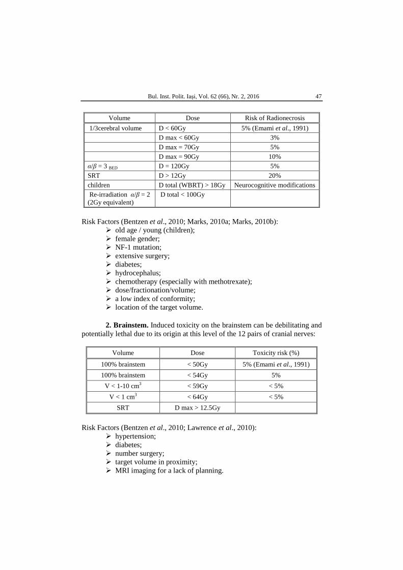
Bul. Inst. Polit. Iaşi, Vol. 62 (66), Nr. 2, 2016 47
Volume Dose Risk of Radionecrosis 1/3cerebral volume D < 60Gy 5% (Emami et al., 1991) D max < 60Gy 3% D max = 70Gy 5% D max = 90Gy 10% α/β = 3 BED D = 120Gy 5% SRT D > 12Gy 20% children D total (WBRT) > 18Gy Neurocognitive modifications Re-irradiation α/β = 2 (2Gy equivalent)
D total < 100Gy
Risk Factors (Bentzen et al., 2010; Marks, 2010a; Marks, 2010b):
old age / young (children); female gender; NF-1 mutation; extensive surgery; diabetes; hydrocephalus; chemotherapy (especially with methotrexate); dose/fractionation/volume; a low index of conformity; location of the target volume.
2. Brainstem. Induced toxicity on the brainstem can be debilitating and potentially lethal due to its origin at this level of the 12 pairs of cranial nerves:
Volume Dose Toxicity risk (%)
100% brainstem < 50Gy 5% (Emami et al., 1991) 100% brainstem < 54Gy 5%
V < 1-10 cm3 < 59Gy < 5% V < 1 cm3 < 64Gy < 5%
SRT D max > 12.5Gy
Risk Factors (Bentzen et al., 2010; Lawrence et al., 2010):
hypertension; diabetes; number surgery; target volume in proximity; MRI imaging for a lack of planning.
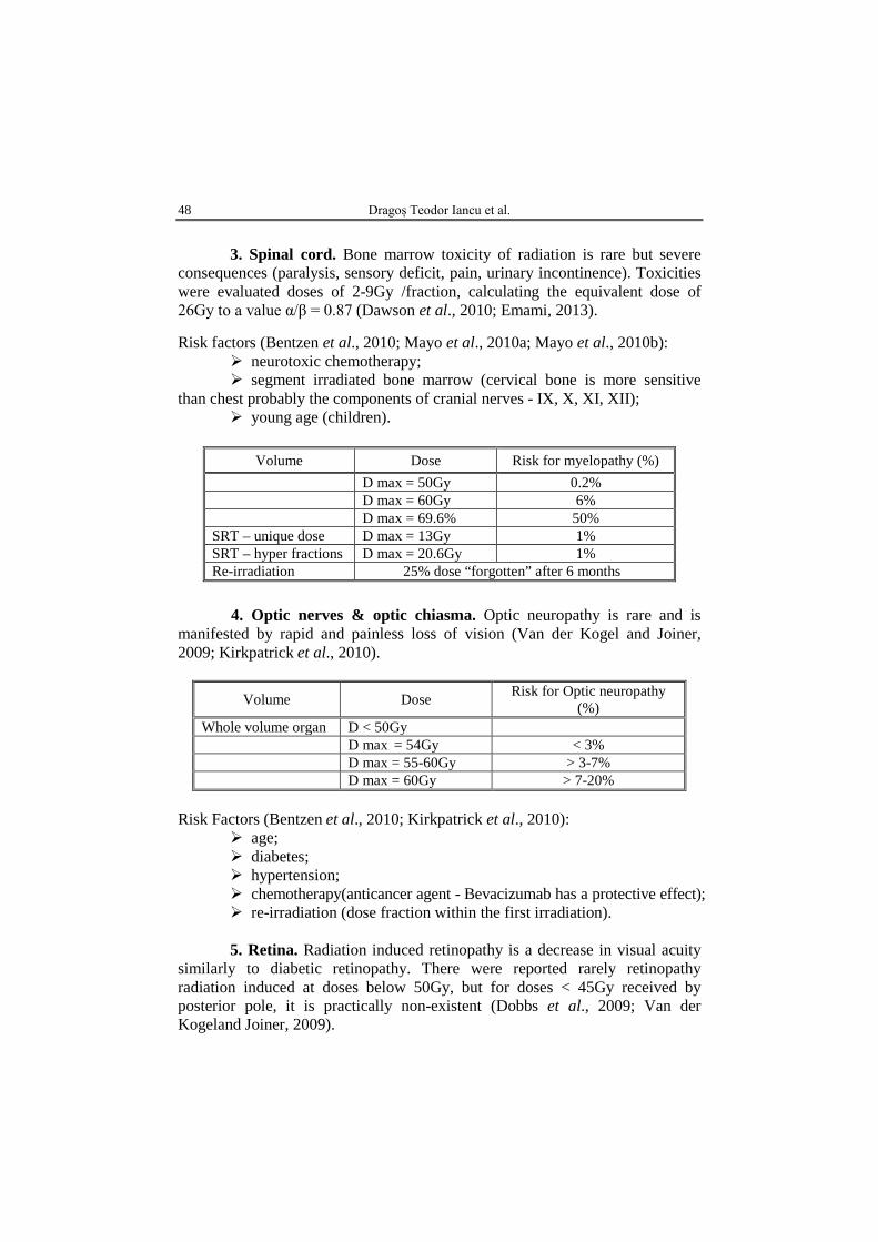
48 Dragoș Teodor Iancu et al.
3. Spinal cord. Bone marrow toxicity of radiation is rare but severe
consequences (paralysis, sensory deficit, pain, urinary incontinence). Toxicities were evaluated doses of 2-9Gy /fraction, calculating the equivalent dose of 26Gy to a value α/β = 0.87 (Dawson et al., 2010; Emami, 2013). Risk factors (Bentzen et al., 2010; Mayo et al., 2010a; Mayo et al., 2010b):
neurotoxic chemotherapy; segment irradiated bone marrow (cervical bone is more sensitive
than chest probably the components of cranial nerves - IX, X, XI, XII); young age (children).
Volume Dose Risk for myelopathy (%)
D max = 50Gy 0.2% D max = 60Gy 6% D max = 69.6% 50% SRT – unique dose D max = 13Gy 1% SRT – hyper fractions D max = 20.6Gy 1% Re-irradiation 25% dose “forgotten” after 6 months
4. Optic nerves & optic chiasma. Optic neuropathy is rare and is
manifested by rapid and painless loss of vision (Van der Kogel and Joiner, 2009; Kirkpatrick et al., 2010).
Volume Dose Risk for Optic neuropathy (%)
Whole volume organ D < 50Gy D max = 54Gy < 3% D max = 55-60Gy > 3-7% D max = 60Gy > 7-20%
Risk Factors (Bentzen et al., 2010; Kirkpatrick et al., 2010):
age; diabetes; hypertension; chemotherapy(anticancer agent - Bevacizumab has a protective effect); re-irradiation (dose fraction within the first irradiation). 5. Retina. Radiation induced retinopathy is a decrease in visual acuity
similarly to diabetic retinopathy. There were reported rarely retinopathy radiation induced at doses below 50Gy, but for doses < 45Gy received by posterior pole, it is practically non-existent (Dobbs et al., 2009; Van der Kogeland Joiner, 2009).
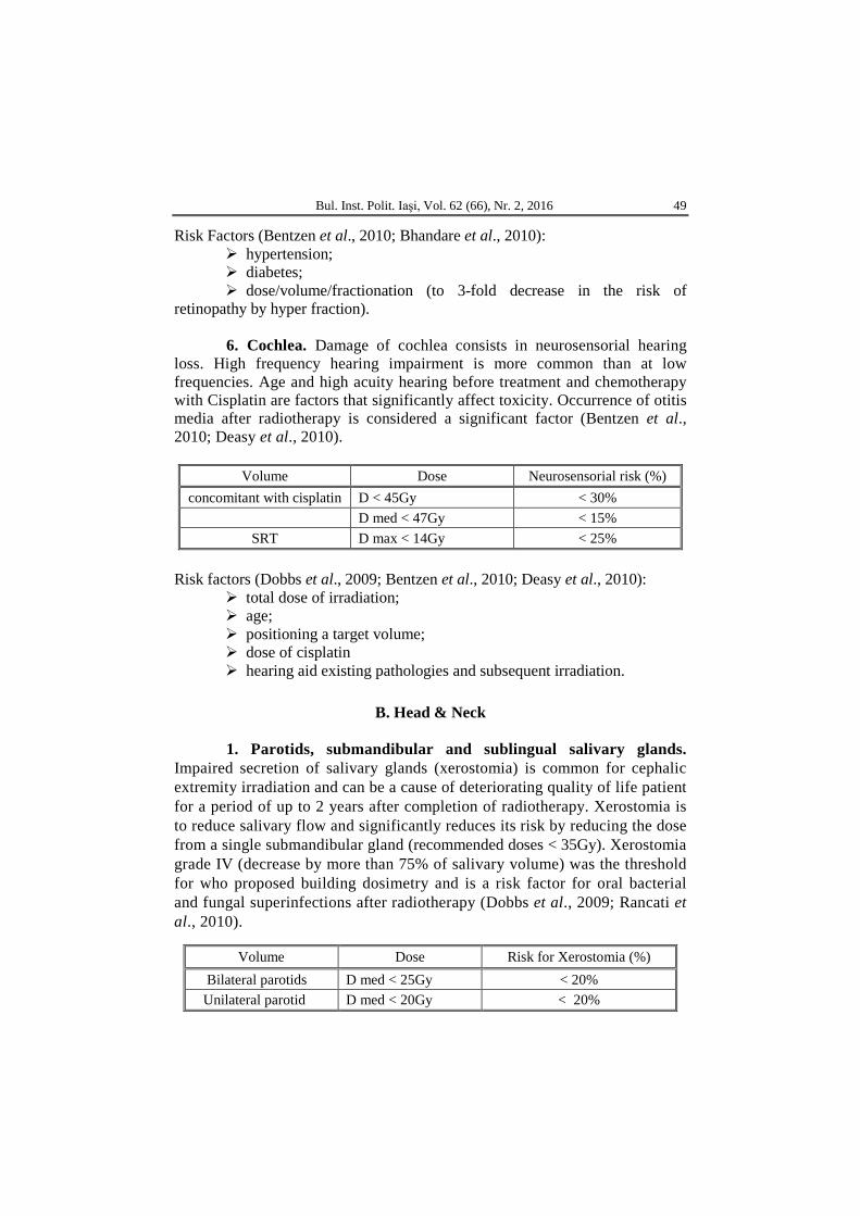
Bul. Inst. Polit. Iaşi, Vol. 62 (66), Nr. 2, 2016 49
Risk Factors (Bentzen et al., 2010; Bhandare et al., 2010): hypertension; diabetes; dose/volume/fractionation (to 3-fold decrease in the risk of
retinopathy by hyper fraction). 6. Cochlea. Damage of cochlea consists in neurosensorial hearing
loss. High frequency hearing impairment is more common than at low frequencies. Age and high acuity hearing before treatment and chemotherapy with Cisplatin are factors that significantly affect toxicity. Occurrence of otitis media after radiotherapy is considered a significant factor (Bentzen et al., 2010; Deasy et al., 2010).
Volume Dose Neurosensorial risk (%)
concomitant with cisplatin D < 45Gy < 30% D med < 47Gy < 15%
SRT D max < 14Gy < 25%
Risk factors (Dobbs et al., 2009; Bentzen et al., 2010; Deasy et al., 2010): total dose of irradiation; age; positioning a target volume; dose of cisplatin hearing aid existing pathologies and subsequent irradiation.
B. Head & Neck
1. Parotids, submandibular and sublingual salivary glands.
Impaired secretion of salivary glands (xerostomia) is common for cephalic extremity irradiation and can be a cause of deteriorating quality of life patient for a period of up to 2 years after completion of radiotherapy. Xerostomia is to reduce salivary flow and significantly reduces its risk by reducing the dose from a single submandibular gland (recommended doses < 35Gy). Xerostomia grade IV (decrease by more than 75% of salivary volume) was the threshold for who proposed building dosimetry and is a risk factor for oral bacterial and fungal superinfections after radiotherapy (Dobbs et al., 2009; Rancati et al., 2010).
Volume Dose Risk for Xerostomia (%) Bilateral parotids D med < 25Gy < 20% Unilateral parotid D med < 20Gy < 20%
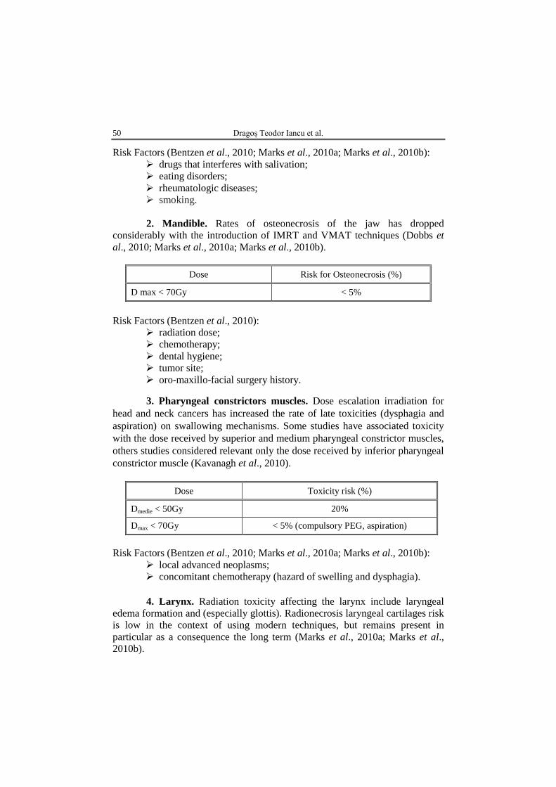
50 Dragoș Teodor Iancu et al.
Risk Factors (Bentzen et al., 2010; Marks et al., 2010a; Marks et al., 2010b): drugs that interferes with salivation; eating disorders; rheumatologic diseases; smoking. 2. Mandible. Rates of osteonecrosis of the jaw has dropped
considerably with the introduction of IMRT and VMAT techniques (Dobbs et al., 2010; Marks et al., 2010a; Marks et al., 2010b).
Dose Risk for Osteonecrosis (%)
D max < 70Gy < 5%
Risk Factors (Bentzen et al., 2010):
radiation dose; chemotherapy; dental hygiene; tumor site; oro-maxillo-facial surgery history.
3. Pharyngeal constrictors muscles. Dose escalation irradiation for head and neck cancers has increased the rate of late toxicities (dysphagia and aspiration) on swallowing mechanisms. Some studies have associated toxicity with the dose received by superior and medium pharyngeal constrictor muscles, others studies considered relevant only the dose received by inferior pharyngeal constrictor muscle (Kavanagh et al., 2010).
Dose Toxicity risk (%)
Dmedie < 50Gy 20%
Dmax < 70Gy < 5% (compulsory PEG, aspiration)
Risk Factors (Bentzen et al., 2010; Marks et al., 2010a; Marks et al., 2010b):
local advanced neoplasms; concomitant chemotherapy (hazard of swelling and dysphagia). 4. Larynx. Radiation toxicity affecting the larynx include laryngeal
edema formation and (especially glottis). Radionecrosis laryngeal cartilages risk is low in the context of using modern techniques, but remains present in particular as a consequence the long term (Marks et al., 2010a; Marks et al., 2010b).
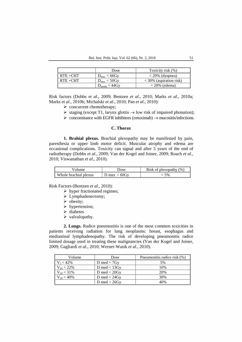
Bul. Inst. Polit. Iaşi, Vol. 62 (66), Nr. 2, 2016 51
Dose Toxicity risk (%)
RTE +CHT Dmax < 66Gy < 20% (dyspnea) RTE +CHT Dmax < 50Gy < 30% (aspiration risk) Dmedie < 44Gy < 20% (edema)
Risk factors (Dobbs et al., 2009; Bentzen et al., 2010; Marks et al., 2010a; Marks et al., 2010b; Michalski et al., 2010; Pan et al., 2010):
concurrent chemotherapy; staging (except T1, larynx glottis → low risk of impaired phonation); concomitance with EGFR inhibitors (cetuximab) → mucositis/infections.
C. Thorax
1. Brahial plexus. Brachial plexopathy may be manifested by pain,
paresthesia or upper limb motor deficit. Muscular atrophy and edema are occasional complications. Toxicity can signal and after 5 years of the end of radiotherapy (Dobbs et al., 2009; Van der Kogel and Joiner, 2009; Roach et al., 2010; Viswanathan et al., 2010).
Volume Dose Risk of plexopathy (%)
Whole brachial plexus D max < 60Gy < 5% Risk Factors (Bentzen et al., 2010):
hyper fractionated regimes; Lymphadenectomy; obesity; hypertension; diabetes valvulopathy.
2. Lungs. Radice pneumonitis is one of the most common toxicities in patients receiving radiation for lung neoplasms: breast, esophagus and mediastinal lymphadenopathy. The risk of developing pneumonitis radice limited dosage used in treating these malignancies (Van der Kogel and Joiner, 2009; Gagliardi et al., 2010; Werner-Wasik et al., 2010).
Volume Dose Pneumonitis radice risk (%)
V5 < 42% D med = 7Gy 5% V20 < 22% D med < 13Gy 10% V20 < 31% D med < 20Gy 20% V20 < 40% D med < 24Gy 30% D med < 26Gy 40%
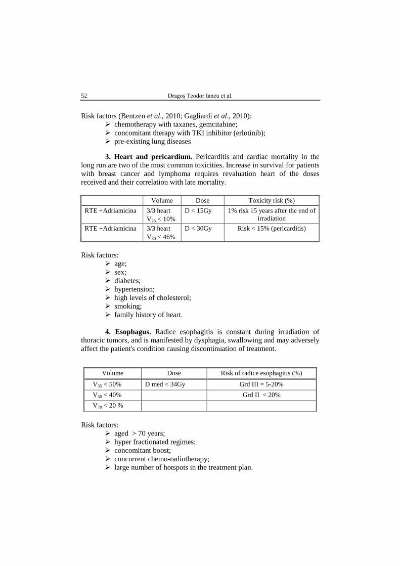
52 Dragoș Teodor Iancu et al.
Risk factors (Bentzen et al., 2010; Gagliardi et al., 2010):
chemotherapy with taxanes, gemcitabine; concomitant therapy with TKI inhibitor (erlotinib); pre-existing lung diseases
3. Heart and pericardium. Pericarditis and cardiac mortality in the long run are two of the most common toxicities. Increase in survival for patients with breast cancer and lymphoma requires revaluation heart of the doses received and their correlation with late mortality.
Volume Dose Toxicity risk (%)
RTE +Adriamicina 3/3 heart V25 < 10%
D < 15Gy 1% risk 15 years after the end of irradiation
RTE +Adriamicina 3/3 heart V30 < 46%
D < 30Gy Risk < 15% (pericarditis)
Risk factors:
age; sex; diabetes; hypertension; high levels of cholesterol; smoking; family history of heart. 4. Esophagus. Radice esophagitis is constant during irradiation of
thoracic tumors, and is manifested by dysphagia, swallowing and may adversely affect the patient's condition causing discontinuation of treatment.
Risk factors:
aged > 70 years; hyper fractionated regimes; concomitant boost; concurrent chemo-radiotherapy; large number of hotspots in the treatment plan.
Volume Dose Risk of radice esophagitis (%)
V35 < 50% D med < 34Gy Grd III = 5-20% V50 < 40% Grd II < 20% V70 < 20 %
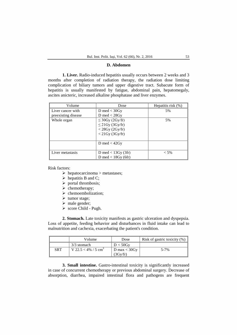
Bul. Inst. Polit. Iaşi, Vol. 62 (66), Nr. 2, 2016 53
D. Abdomen 1. Liver. Radio-induced hepatitis usually occurs between 2 weeks and 3
months after completion of radiation therapy, the radiation dose limiting complication of biliary tumors and upper digestive tract. Subacute form of hepatitis is usually manifested by fatigue, abdominal pain, hepatomegaly, ascites anicteric, increased alkaline phosphatase and liver enzymes.
Volume Dose Hepatitis risk (%)
Liver cancer with preexisting disease
D med < 30Gy D med < 28Gy
5%
Whole organ ≤ 30Gy (2Gy/fr) ≤ 21Gy (3Gy/fr) < 28Gy (2Gy/fr) < 21Gy (3Gy/fr)
5%
D med < 42Gy
Liver metastasis D med < 13Gy (3fr) D med < 18Gy (6fr)
< 5%
Risk factors:
hepatocarcinoma > metastases; hepatitis B and C; portal thrombosis; chemotherapy; chemoembolization; tumor stage; male gender; score Child - Pugh. 2. Stomach. Late toxicity manifests as gastric ulceration and dyspepsia.
Loss of appetite, feeding behavior and disturbances in fluid intake can lead to malnutrition and cachexia, exacerbating the patient's condition.
Volume Dose Risk of gastric toxicity (%) 3/3 stomach D < 50Gy SRT V 22.5 < 4% / 5 cm3 D max < 30Gy
(3Gy/fr) 5-7%
3. Small intestine. Gastro-intestinal toxicity is significantly increased
in case of concurrent chemotherapy or previous abdominal surgery. Decrease of absorption, diarrhea, impaired intestinal flora and pathogens are frequent
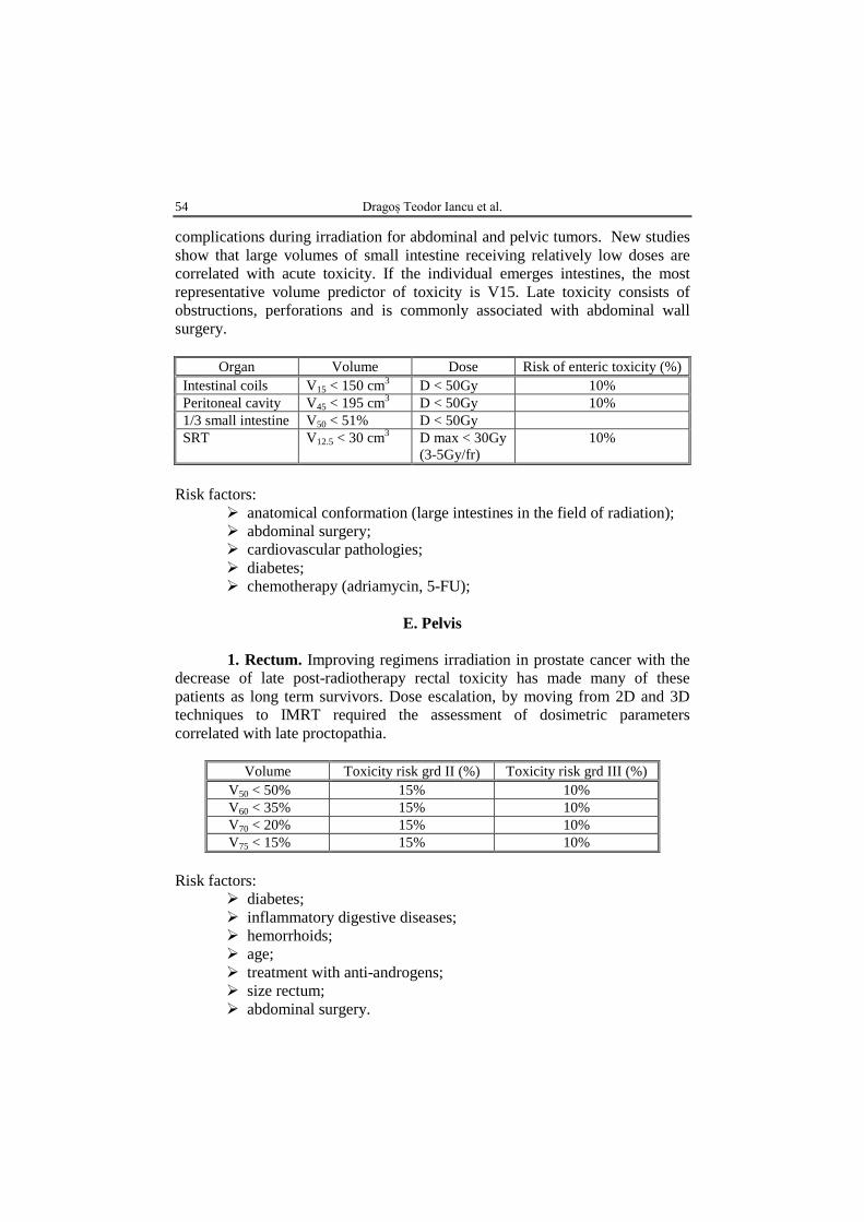
54 Dragoș Teodor Iancu et al.
complications during irradiation for abdominal and pelvic tumors. New studies show that large volumes of small intestine receiving relatively low doses are correlated with acute toxicity. If the individual emerges intestines, the most representative volume predictor of toxicity is V15. Late toxicity consists of obstructions, perforations and is commonly associated with abdominal wall surgery.
Organ Volume Dose Risk of enteric toxicity (%)
Intestinal coils V15 < 150 cm3 D < 50Gy 10% Peritoneal cavity V45 < 195 cm3 D < 50Gy 10% 1/3 small intestine V50 < 51% D < 50Gy SRT V12.5 < 30 cm3 D max < 30Gy
(3-5Gy/fr) 10%
Risk factors:
anatomical conformation (large intestines in the field of radiation); abdominal surgery; cardiovascular pathologies; diabetes; chemotherapy (adriamycin, 5-FU);
E. Pelvis 1. Rectum. Improving regimens irradiation in prostate cancer with the
decrease of late post-radiotherapy rectal toxicity has made many of these patients as long term survivors. Dose escalation, by moving from 2D and 3D techniques to IMRT required the assessment of dosimetric parameters correlated with late proctopathia.
Volume Toxicity risk grd II (%) Toxicity risk grd III (%)
V50 < 50% 15% 10% V60 < 35% 15% 10% V70 < 20% 15% 10% V75 < 15% 15% 10%
Risk factors:
diabetes; inflammatory digestive diseases; hemorrhoids; age; treatment with anti-androgens; size rectum; abdominal surgery.

Bul. Inst. Polit. Iaşi, Vol. 62 (66), Nr. 2, 2016 55
2. Bladder elasticity makes difficult a performing dosimetric analysis with predictive toxicity. Affecting the entire body may be manifested by dysuria, urinary frequency, bladder spasm, reducing the flow urinary incontinence. Damage is focal manifestations: hematuria, fistula, obstruction, ulceration and necrosis. Risk factors:
hormone therapy; chemotherapy (cyclophosphamide); TUR-V&TUR-P; underlying genitourinary pathology; hysterectomy; obesity; smoking; black race; age; diabetes.
3. Kidney. Renal dysfunction after radiotherapy can cause symptoms and biochemical and radiological changes form. High latency ranges are as renal toxicity late to be undervalued. Most studies have evaluated serum creatinine clearance decreased in relation to the dose received by both kidneys. Risk factors:
renal failure; diabetes; cardiac pathologies; smoking.
4. Penile bulb. Erectile dysfunction can be a cause of discomfort for
patients with prostate cancer. The dose received by the penile bulb is considered a predictor.
Risk factors:
age; diabetes; treatment with anti-androgens; hypertension; smoking
Volume Dose Toxicity risk (%) V60-V70 < 70Gy D med < 52Gy < 55% V90 < 50Gy D med 95% din gland < 50Gy < 35%
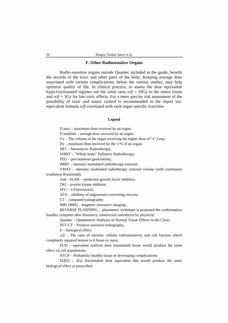
56 Dragoș Teodor Iancu et al.
F. Other Radiosensitive Organs
Radio-sensitive organs outside Quantec included in the guide, benefit the records of the toxic and other parts of the body. Keeping average dose associated with various complications, below the various studies, may help optimize quality of life. In clinical practice, to assess the dose equivalent hypo-fractionated regimes use the value ratio α/β = 10Gy to the tumor tissue and α/β = 3Gy for late toxic effects. For a more precise risk assessment of the possibility of toxic and tumor control is recommended in the report izo-equivalent formula α/β correlated with each organ specific toxicities
Legend
D max – maximum dose received by an organ; D medium – average dose received by an organ; Vx – The volume of the organ receiving the higher dose of "x" Gray; Dy – minimum dose received by the 'y'% of an organ; SRT – Stereotactic Radiotherapy; WBRT – "Whole brain" Palliative Radiotherapy; PEG – percutaneous gastrostomy; IMRT – intensity modulated radiotherapy external; VMAT – intensity modulated radiotherapy external volume (with continuous
irradiation Rotational); Anti - EGFR – epidermal growth factor inhibitor; TKI – tyrozin kinase inhibitor; 5FU – 5-Fluorouracil; ACE – inhibitor of angiotensin converting enzyme; CT – computed tomography; MRI (MRI) – magnetic resonance imaging; REVERSE PLANNING – planimetric technique is proposed the conformation
bundles computer after dosimetry constriction introduced by physicist; Quantec – Quantitative Analyses of Normal Tissue Effects in the Clinic; PET-CT – Positron emission tomography; E – biological effect; α/β – The ratio of intrinsic cellular radiosensitivity and cell fraction which
completely repaired lesions in 6 hours or more; EUD – equivalent uniform dose transmitted tissue would produce the same
effect on cell populations; NTCP – Probability healthy tissue of developing complications; EQD2 – 2Gy fractionated dose equivalent that would produce the same
biological effect as prescribed.
Bul. Inst. Polit. Iaşi, Vol. 62 (66), Nr. 2, 2016 57
REFERENCES
Bentzen S.M., Constine L.S., Deasy J.O., Quantitative Analyses of Normal Tissue
Effects in the Clinic (QUANTEC): An Introduction to the Scientific Issues, Int. J. Radiat. Oncol. Biol. Phys., 2010, 76, 3, Suppl., S3-9, doi: 10.1016/j.ijrobp.2009.09.040.
Bhandare N., Jackson A., Eisbruch A. et al., Radiation Therapu and Hearing Loss, Int. J. Radiat. Oncol. Biol. Phys. 2010, 76, 3, Suppl., S50–S57, doi: 10.1016/j.ijrobp.2009.04.096.
Bortfeld T., Schmidt-Ullrich R., De Neve W., Wazer D.E., Image-Guided IMRT, Berlin, Heidelberg, Springer, 2006.
Dawson L.A., Kavanagh B.D., Paulino A.C. et al., Radiation-Associated Kidney Injury, Int. J. Radiat. Oncol. Biol. Phys., 2010, 76, 3, Suppl., S108-115, doi: 10.1016/j.ijrobp.2009.02.089.
Deasy J.O., Moiseenko V., Marks L. et al., Radiotherapy Dose-Volume Effects on Salivary Gland Function, Int. J. Radiat. Oncol. Biol. Phys., 2010, 76, 3, Suppl., S58-63, doi: 10.1016/j.ijrobp.2009.06.090.
Dobbs J.E., Barrett A., Roques T., Practical Radiotherapy Planning, Fourth Edition, Boca Raton, Florida, CRC Press, 2009.
Emami B., Lyman J., Brown A. et al., Tolerance of Normal Tissue to Therapeutic Irradiation, Int. J. Radiat. Oncol. Biol. Phys., 21, 1, 109-122 (1991).
Emami B., Tolerance of Normal Tissue to Therapeutic Radiation, Reports of Radiotherapy and Oncology, 2013, Vol. 1, No. 1, 36-48.
Gagliardi G., Constine L.S., Moiseenko V. et al., Radiation Dose-Volume Effects in the Heart, Int. J. Radiat. Oncol. Biol. Phys., 2010, 76, 3, Suppl., S77-85, doi: 10.1016/j.ijrobp.2009.04.093.
Hayes W.A., Kruger C.L., Principles and Methods of Toxicology, 5 Edition, Boca Raton, Florida, CRC Press, 2007.
Kavanagh B.D., Pan C.C., Dawson L.A. et al., Radiation Dose-Volume Effects in the Stomach and Small Bowel, Int. J. Radiat. Oncol. Biol. Phys., 2010, 76, 3, Suppl., S101-107, doi: 10.1016/j.ijrobp.2009.05.071.
Kirkpatrick J.P., van der Kogel A.J., Schultheiss T.E., Radiation Dose-Volume Effects in the Spinal Cord, Int. J. Radiat. Oncol. Biol. Phys., 2010, 76, 3, Suppl., S42-49, doi: 10.1016/j.ijrobp.2009.04.095.
Lawrence Y.R., Li X.A., el Naqa I. et al., Radiation Dose-Volume Effects in the Brain, Int. J. Radiat. Oncol. Biol. Phys., 2010, 76, 3, Suppl., S20-27, doi: 11.1016/j.ijrobp.2009.02.091.
Marks L.B., Yorke E.D., Jackson A. et al., Use of Normal Tissue Complication Probability Models in the Clinic, Int. J. Radiat. Oncol. Biol. Phys., 2010, 76, 3, Suppl., S10-19, doi: 10.1016/j.ijrobp.2009.07.1754.
Marks L.B., Bentzen S.M., Deasy J.O. et al., Radiation Dose-Volume Effects in the Lung, Int. J. Radiat. Oncol. Biol. Phys., 2010, 76, 3, Suppl., S70-76, doi: 10.1016/j.ijrobp.2009.06.091.
Mayo C., Martel M.K., Marks L.B. et al., Radiation Dose-Volume Effects of Optic Nerves and Chiasm, Int. J. Radiat. Oncol. Biol. Phys., 2010, 76, 3, Suppl., S28-35, doi: 10.1016/j.ijrobp.2009.07.1753.
58 Dragoș Teodor Iancu et al.
Mayo C., Yorke E., Merchant T.E., Radiation Associated Brainstem Injury, Int. J. Radiat. Oncol. Biol. Phys., 2010, 76, 3, Suppl., S36-S41, doi: 10.1016/j.ijrobp.2009.08.078
Michalski J.M., Gay H., Jackson A. et al., Radiation Dose-Volume Effects in Radiation-Induced Rectal Injury, Int. J. Radiat. Oncol. Biol. Phys., 2010, 76, 3, Suppl., S123-129, doi: 10.1016/j.ijrobp.2009.03.078.
Nishimura Y., Komaki R., Intensity-Modulated Radiation Therapy, Clinical Evidence and Techniques, Tokio, Springer, 2015.
Pan C.C., Kavanagh B.D, Dawson L.A. et al., Radiation-Associated Liver Injury, Int. J. Radiat. Oncol. Biol. Phys., 2010, 76, 3, Suppl., S94-100, doi: 0.1016/j.ijrobp.2009.06.092.
Rancati T., Schwarz M., Allen A.M., Radiation Dose-Volume Effects in the Larynx and Pharynx, Int. J. Radiat. Oncol. Biol. Phys., 2010, 76, 3, Suppl., S64-69, doi: 10.1016/j.ijrobp.2009.03.079.
Roach M., Nam J., Gagliardi G. et al., Radiation Dose-Volume Effects and the Penile Bulb, Int. J. Radiat. Oncol. Biol. Phys., 2010, 76, 3, Suppl., S130-134, doi: 10.1016/j.ijrobp.2009.04.094.
Rubin P., Constine L.S., Marks L.B., ALERT ‒ Adverse Late Effects of Cancer Treatment, Vol. 1, General Concepts and Specific Precepts, Vol. 2, Normal Tissue Specific Sites and Systems New York, Springer, 2014.
Schwartz C.L., Hobbie W.L., Constine L.S., Ruccione K.S., Survivors of Childhood and Adolescent Cancer, A Multidisciplinary Approach, Heidelberg, Springer-Verlag, 2005.
Van der Kogel A., Joiner M., Basic Clinical Radiobiology, 4th Edition, London, Hodder Arnold Publication, 2009.
Viswanathan A.N., Yorke E.D., Marks L.B. et al., Radiation Dose-Volume Effects of the Urinary Bladder, Int. J. Radiat. Oncol. Biol. Phys., 2010, 76, 3, Suppl., S116-122, doi: 10.1016/j.ijrobp.2009.02.090.
Werner-Wasik M., Yorke E., Deasy J. et al., Radiation Dose-Volume Effects in the Esophagus, Int. J. Radiat. Oncol. Biol. Phys., 2010, 76, 3, Suppl., S86-93, doi: 10.1016/j.ijrobp.2009.05.070.
DOZA TOTALĂ CORELATĂ CU VOLUMUL TUMORAL ȘI RISCUL DE TOXICITATE ÎN RADIOTERAPIA MODERNĂ
(Rezumat)
Radioterapia este o componentă esențială și inseparabilă în contextul
tratamentului multidisciplinar al cancerului. Se estimează că aproximativ 70% dintre pacienții cu cancer ar putea beneficia de radioterapie pentru tratamentul bolii localizate, controlul local și paliativ. Cu toate acestea, în planificarea și implementarea secvențelor terapeutice oncologice, radioterapia este frecvent ultima resursă care se ia în considerare.
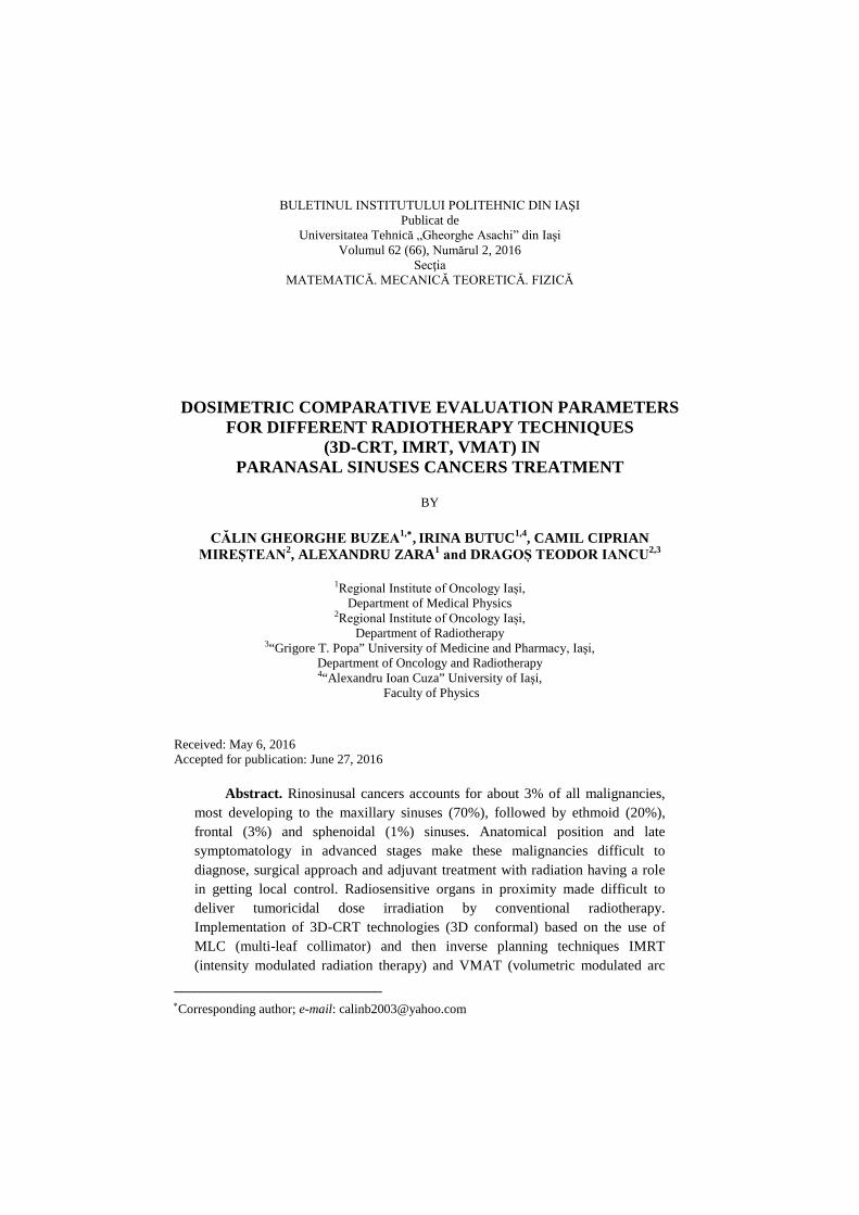
BULETINUL INSTITUTULUI POLITEHNIC DIN IAŞI Publicat de
Universitatea Tehnică „Gheorghe Asachi” din Iaşi Volumul 62 (66), Numărul 2, 2016
Secţia MATEMATICĂ. MECANICĂ TEORETICĂ. FIZICĂ
DOSIMETRIC COMPARATIVE EVALUATION PARAMETERS FOR DIFFERENT RADIOTHERAPY TECHNIQUES
(3D-CRT, IMRT, VMAT) IN PARANASAL SINUSES CANCERS TREATMENT
BY
CĂLIN GHEORGHE BUZEA1,∗, IRINA BUTUC1,4, CAMIL CIPRIAN
MIREȘTEAN2, ALEXANDRU ZARA1 and DRAGOȘ TEODOR IANCU2,3
1Regional Institute of Oncology Iași,
Department of Medical Physics 2Regional Institute of Oncology Iași,
Department of Radiotherapy 3“Grigore T. Popa” University of Medicine and Pharmacy, Iaşi,
Department of Oncology and Radiotherapy 4“Alexandru Ioan Cuza” University of Iaşi,
Faculty of Physics
Received: May 6, 2016 Accepted for publication: June 27, 2016
Abstract. Rinosinusal cancers accounts for about 3% of all malignancies,
most developing to the maxillary sinuses (70%), followed by ethmoid (20%), frontal (3%) and sphenoidal (1%) sinuses. Anatomical position and late symptomatology in advanced stages make these malignancies difficult to diagnose, surgical approach and adjuvant treatment with radiation having a role in getting local control. Radiosensitive organs in proximity made difficult to deliver tumoricidal dose irradiation by conventional radiotherapy. Implementation of 3D-CRT technologies (3D conformal) based on the use of MLC (multi-leaf collimator) and then inverse planning techniques IMRT (intensity modulated radiation therapy) and VMAT (volumetric modulated arc
∗Corresponding author; e-mail: [email protected]
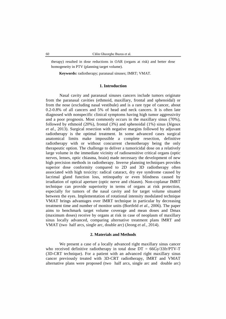
60 Călin Gheorghe Buzea et al.
therapy) resulted in dose reductions in OAR (organs at risk) and better dose homogeneity in PTV (planning target volume).
Keywords: radiotherapy; paranasal sinuses; IMRT; VMAT.
1. Introduction Nasal cavity and paranasal sinuses cancers include tumors originate
from the paranasal cavities (ethmoid, maxillary, frontal and sphenoidal) or from the nose (excluding nasal vestibule) and is a rare type of cancer, about 0.2-0.8% of all cancers and 5% of head and neck cancers. It is often late diagnosed with nonspecific clinical symptoms having high tumor aggressivity and a poor prognosis. Most commonly occurs in the maxillary sinus (70%), followed by ethmoid (20%), frontal (3%) and sphenoidal (1%) sinus (Jégoux et al., 2013). Surgical resection with negative margins followed by adjuvant radiotherapy is the optimal treatment. In some advanced cases surgical anatomical limits make impossible a complete resection, definitive radiotherapy with or without concurrent chemotherapy being the only therapeutic option. The challenge to deliver a tumoricidal dose on a relatively large volume in the immediate vicinity of radiosensitive critical organs (optic nerves, lenses, optic chiasma, brain) made necessary the development of new high precision methods in radiotherapy. Inverse planning techniques provides superior dose conformity compared to 2D and 3D radiotherapy often associated with high toxicity: radical cataract, dry eye syndrome caused by lacrimal gland function loss, retinopathy or even blindness caused by irradiation of optical aperture (optic nerve and chiasm). Non-coplanar IMRT technique can provide superiority in terms of organs at risk protection, especially for tumors of the nasal cavity and for target volume situated between the eyes. Implementation of rotational intensity modulated technique VMAT brings advantages over IMRT technique in particular by decreasing treatment time and number of monitor units (Bortfeld et al., 2006). The paper aims to benchmark target volume coverage and mean doses and Dmax (maximum doses) receive by organs at risk in case of neoplasm of maxillary sinus locally advanced, comparing alternative treatment plans IMRT and VMAT (two half arcs, single arc, double arc) (Jeong et al., 2014).
2. Materials and Methods
We present a case of a locally advanced right maxillary sinus cancer
who received definitive radiotherapy in total dose DT = 66Gy/33fr/PTV-T (3D-CRT technique). For a patient with an advanced right maxillary sinus cancer previously treated with 3D-CRT radiotherapy, IMRT and VMAT alternative plans were proposed (two half arcs, single arc and double arc)
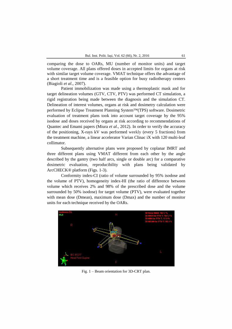
Bul. Inst. Polit. Iaşi, Vol. 62 (66), Nr. 2, 2016 61
comparing the dose to OARs, MU (number of monitor units) and target volume coverage. All plans offered doses in accepted limits for organs at risk with similar target volume coverage. VMAT technique offers the advantage of a short treatment time and is a feasible option for busy radiotherapy centers (Biagioli et al., 2007).
Patient immobilization was made using a thermoplastic mask and for target delineation volumes (GTV, CTV, PTV) was performed CT simulation, a rigid registration being made between the diagnosis and the simulation CT. Delineation of interest volumes, organs at risk and dosimetry calculation were performed by Eclipse Treatment Planning System™(TPS) software. Dosimetric evaluation of treatment plans took into account target coverage by the 95% isodose and doses received by organs at risk according to recommendations of Quantec and Emami papers (Miura et al., 2012). In order to verify the accuracy of the positioning, X-rays kV was performed weekly (every 5 fractions) from the treatment machine, a linear accelerator Varian Clinac iX with 120 multi-leaf collimator.
Subsequently alternative plans were proposed by coplanar IMRT and three different plans using VMAT different from each other by the angle described by the gantry (two half arcs, single or double arc) for a comparative dosimetric evaluation, reproducibility with plans being validated by ArcCHECK® platform (Figs. 1-3).
Conformity index-CI (ratio of volume surrounded by 95% isodose and the volume of PTV), homogeneity index-HI (the ratio of difference between volume which receives 2% and 98% of the prescribed dose and the volume surrounded by 50% isodose) for target volume (PTV), were evaluated together with mean dose (Dmean), maximum dose (Dmax) and the number of monitor units for each technique received by the OARs.
Fig. 1 ‒ Beam orientation for 3D-CRT plan.
62 Călin Gheorghe Buzea et al.
Fig. 2 ‒ Beam orientation for IMRT plan.
Fig. 3 ‒ Half arc radiotherapy plan – beam angle rotation and isodose curves.
3. Results
All doses received by organs at risk using IMRT and VMAT techniques
(two half arcs, single arc, double arc) were compared to the dose received by the same organs in 3D-CRT technique (Fig. 4).
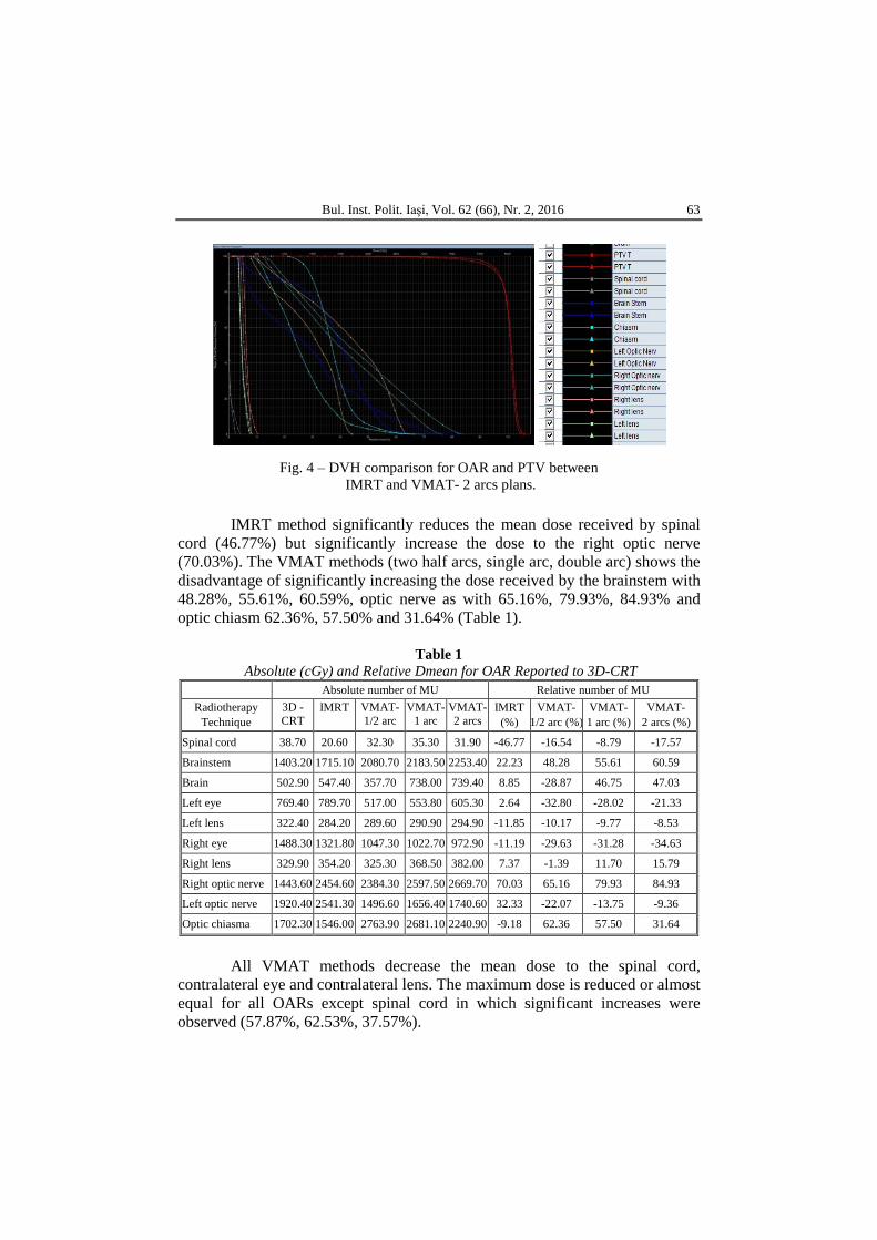
Bul. Inst. Polit. Iaşi, Vol. 62 (66), Nr. 2, 2016 63
Fig. 4 ‒ DVH comparison for OAR and PTV between IMRT and VMAT- 2 arcs plans.
IMRT method significantly reduces the mean dose received by spinal
cord (46.77%) but significantly increase the dose to the right optic nerve (70.03%). The VMAT methods (two half arcs, single arc, double arc) shows the disadvantage of significantly increasing the dose received by the brainstem with 48.28%, 55.61%, 60.59%, optic nerve as with 65.16%, 79.93%, 84.93% and optic chiasm 62.36%, 57.50% and 31.64% (Table 1).
Table 1
Absolute (cGy) and Relative Dmean for OAR Reported to 3D-CRT Absolute number of MU Relative number of MU
Radiotherapy Technique
3D -CRT
IMRT VMAT- 1/2 arc
VMAT- 1 arc
VMAT- 2 arcs
IMRT (%)
VMAT- 1/2 arc (%)
VMAT- 1 arc (%)
VMAT- 2 arcs (%)
Spinal cord 38.70 20.60 32.30 35.30 31.90 -46.77 -16.54 -8.79 -17.57
Brainstem 1403.20 1715.10 2080.70 2183.50 2253.40 22.23 48.28 55.61 60.59
Brain 502.90 547.40 357.70 738.00 739.40 8.85 -28.87 46.75 47.03
Left eye 769.40 789.70 517.00 553.80 605.30 2.64 -32.80 -28.02 -21.33
Left lens 322.40 284.20 289.60 290.90 294.90 -11.85 -10.17 -9.77 -8.53
Right eye 1488.30 1321.80 1047.30 1022.70 972.90 -11.19 -29.63 -31.28 -34.63
Right lens 329.90 354.20 325.30 368.50 382.00 7.37 -1.39 11.70 15.79
Right optic nerve 1443.60 2454.60 2384.30 2597.50 2669.70 70.03 65.16 79.93 84.93
Left optic nerve 1920.40 2541.30 1496.60 1656.40 1740.60 32.33 -22.07 -13.75 -9.36
Optic chiasma 1702.30 1546.00 2763.90 2681.10 2240.90 -9.18 62.36 57.50 31.64
All VMAT methods decrease the mean dose to the spinal cord,
contralateral eye and contralateral lens. The maximum dose is reduced or almost equal for all OARs except spinal cord in which significant increases were observed (57.87%, 62.53%, 37.57%).
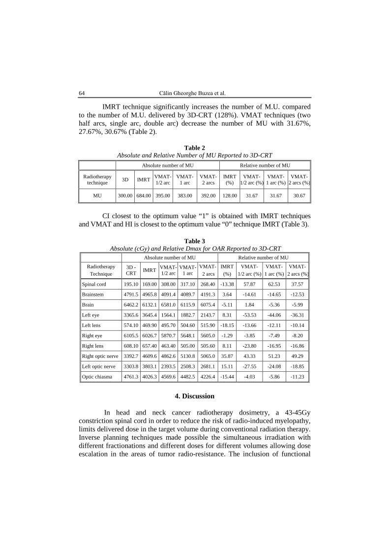
64 Călin Gheorghe Buzea et al.
IMRT technique significantly increases the number of M.U. compared to the number of M.U. delivered by 3D-CRT (128%). VMAT techniques (two half arcs, single arc, double arc) decrease the number of MU with 31.67%, 27.67%, 30.67% (Table 2).
Table 2 Absolute and Relative Number of MU Reported to 3D-CRT
CI closest to the optimum value “1” is obtained with IMRT techniques
and VMAT and HI is closest to the optimum value “0” technique IMRT (Table 3).
Table 3 Absolute (cGy) and Relative Dmax for OAR Reported to 3D-CRT
Absolute number of MU Relative number of MU
Radiotherapy Technique
3D -CRT IMRT VMAT-
1/2 arc VMAT-
1 arc VMAT- 2 arcs
IMRT (%)
VMAT- 1/2 arc (%)
VMAT- 1 arc (%)
VMAT- 2 arcs (%)
Spinal cord 195.10 169.00 308.00 317.10 268.40 -13.38 57.87 62.53 37.57
Brainstem 4791.5 4965.8 4091.4 4089.7 4191.3 3.64 -14.61 -14.65 -12.53
Brain 6462.2 6132.1 6581.0 6115.9 6075.4 -5.11 1.84 -5.36 -5.99
Left eye 3365.6 3645.4 1564.1 1882.7 2143.7 8.31 -53.53 -44.06 -36.31
Left lens 574.10 469.90 495.70 504.60 515.90 -18.15 -13.66 -12.11 -10.14
Right eye 6105.5 6026.7 5870.7 5648.1 5605.0 -1.29 -3.85 -7.49 -8.20
Right lens 608.10 657.40 463.40 505.00 505.60 8.11 -23.80 -16.95 -16.86
Right optic nerve 3392.7 4609.6 4862.6 5130.8 5065.0 35.87 43.33 51.23 49.29
Left optic nerve 3303.8 3803.1 2393.5 2508.3 2681.1 15.11 -27.55 -24.08 -18.85
Optic chiasma 4761.3 4026.3 4569.6 4482.5 4226.4 -15.44 -4.03 -5.86 -11.23
4. Discussion
In head and neck cancer radiotherapy dosimetry, a 43-45Gy
constriction spinal cord in order to reduce the risk of radio-induced myelopathy, limits delivered dose in the target volume during conventional radiation therapy. Inverse planning techniques made possible the simultaneous irradiation with different fractionations and different doses for different volumes allowing dose escalation in the areas of tumor radio-resistance. The inclusion of functional
Absolute number of MU Relative number of MU
Radiotherapy technique 3D IMRT VMAT-
1/2 arc VMAT-
1 arc VMAT- 2 arcs
IMRT (%)
VMAT- 1/2 arc (%)
VMAT- 1 arc (%)
VMAT- 2 arcs (%)
MU 300.00 684.00 395.00 383.00 392.00 128.00 31.67 31.67 30.67
Bul. Inst. Polit. Iaşi, Vol. 62 (66), Nr. 2, 2016 65
imaging PET-CT and diffusion MRI combined with a high-resolution structural imaging could bring benefit in dose escalation.
Basic treatment leads to local failure in 70%. Salvage therapy has a success rate of 30-40% off in head and neck cancers but few patients will be long-time survivors. Re-irradiation and chemo-radiotherapy using IMRT technique are feasible options decreasing the risk of medullary toxicity.
Miura and collaborators have obtained a dose reduction for brainstem and brain by using half-arc VMAT radiotherapy. Similar results were obtained in the case presented for half-arc VMAT method. 3D and IMRT technique still offers best dose solutions for the brainstem but 2 half-arcs VMAT method offers the lowest mean dose for the brain.
For advanced cases involving large irregularly shaped, requiring elective lymph node irradiation, non-coplanar IMRT and VMAT techniques offers dosimetric advantages but clinical benefits will be validated in the future (Orlandi et al., 2014).
5. Conclusions
VMAT technique offers a rapid option with comparable dosimetric
results and coverage of the target volume in maxillary sinus cancer. By significantly reducing the dose to the spinal cord compared to 3D-CRT, IMRT can be used in selected cases for dose escalation in order to improve local control. Saving machine-time can be an advantage for choosing VMAT in crowded radiotherapy centers.
REFERENCES Biagioli M.C., Harvey M., Roman E. et al., Intensity-Modulated Radiotherapy with
Concurrent Chemotherapy for Previously Irradiated, Recurrent Head and Neck Cancer, Int. J. Radiat Oncol Biol Phys., 69, 4, 1067-1073 (2007).
Bortfeld Th., Schmidt-Ullrich R., De Neve W., Wazer D.E., Image-Guided IMRT, Springer-Verlag, Berlin, Heidelberg (2006).
Jégoux F., Métreau A., Louvel G. et al., Paranasal Sinus Cancer, Eur. Ann. Otorhinolaryngol Head Neck Dis., 130, 6, 327-335 (2013).
Jeong Y., Lee S., Kwak J. et al., A Dosimetric Comparison of Volumetric Modulated Arc Therapy (VMAT) and Non-Coplanar Intensity Modulated Radiotherapy (IMRT) for Nasal Cavity and Paranasal Sinus Cancer, Jeong et al., Radiation Oncology, 9,193, 2014.
Miura H., Fujiwara M., Tanooka M. et al., Dosimetric and Delivery Characterizations of Full-Arc and Half-Arc Volumetric-Modulated Arc Therapy for Maxillary Cancer, J. Radiat. Res., 53, 5, 785-790 (2012).
Orlandi E., Giandini T., Iannacone E. et al., Radiotherapy for Un-Resectable Sinonasal Cancers: Dosimetric Comparison of Intensity Modulated Radiation Therapy with Coplanar and Non-Coplanar Volumetric Modulated Arc Therapy, Radiother. Oncol., 113, 2, 260-266, 2014.

66 Călin Gheorghe Buzea et al.
EVALUARE DOZIMETRICĂ COMPARATIVĂ A
DIFERITELOR TEHNICI DE RADIOTERAPIE (3D-CRT, IMRT, VMAT) ÎN TRATAMENTUL CANCERELOR RINOSINUSALE
(Rezumat)
Cancerele rinosinusale reprezintă aproximativ 3% din totalul afecțiunilor
maligne, majoritatea dezvoltându-se la nivelul sinusurilor maxilare (70%), urmate de etmoid (20%), sinusurile frontale (3%) și sfenoidale (1%). Poziția anatomică și simptomatologia tardivă fac ca aceste tumori maligne să fie dificil de diagnosticat, adesea fiind descoperite în stadii avansate. Abordul chirurgical și tratamentul adjuvant cu radiații are un rol esențial în obținerea controlului local. Organele radiosensibile aflate în proximitate fac dificilă livrarea unor doze de iradiere tumoricidale prin radioterapia convențională. Implementarea tehnologiilor 3D-CRT (3D conformațional), bazate pe utilizarea MLC (colimator multi - lamă) și apoi a tehnicilor de planificare inversă IMRT (terapie cu radiații modulate în intensitate) și VMAT (terapie în arc modulată volumetric) a condus la reducerea dozelor la OAR (organe la risc) și o mai bună omogenitate a dozei în PTV (volumul țintă planificat).
BULETINUL INSTITUTULUI POLITEHNIC DIN IAŞI Publicat de
Universitatea Tehnică „Gheorghe Asachi” din Iaşi Volumul 62 (66), Numărul 2, 2016
Secţia MATEMATICĂ. MECANICĂ TEORETICĂ. FIZICĂ
DOSIMETRIC INFLUENCE OF SYSTEMATIC POSITIONING ERRORS BY INDUCING A 3 mm BIAXIAL SHIFT IN A CASE
OF LOCALLY ADVANCED NASOPHARYNX CANCER TREATED WITH EXTERNAL BEAM RADIOTHERAPY
BY
CAMIL CIPRIAN MIREȘTEAN1, CĂLIN GHEORGHE BUZEA2,∗,
ALEXANDRU ZARA2, IRINA BUTUC2,3 and DRAGOȘ TEODOR IANCU1,4
1Regional Institute of Oncology Iași,
Department of Radiotherapy 2Regional Institute of Oncology Iași,
Department of Medical Physics 3“Alexandru Ioan Cuza” University of Iaşi,
Faculty of Physics
4“Grigore T. Popa” University of Medicine and Pharmacy, Iaşi, Department of Oncology and Radiotherapy
Received: May 9, 2016 Accepted for publication: June 30, 2016
Abstract. Head & neck malignancy are cancers where radiotherapy is often the main method of treatment especially in advanced cases outdated for surgery. To analyze the dosimetric effects of a biaxial 3 mm position change from isocenter a + 3 mm shift on the X and Y axes was applied. Doses received by OAR (organs at risk) and target volumes treated with sequential boost were evaluated - PTV-T (target volume of the primary tumor) which received 70Gy/35 fractions, PTV-N66 witch received 66Gy/33 fractions and PTV-N50 irradiated with 50Gy/25 fractions. Evaluation of Dmax, Dmin and Dmean was done both for target volumes and for OAR’s before and after applying the biaxial shift for 3D-CRT(3D-conformal) plans and IMRT (intensity modulated radiation therapy) and VMAT (volumetric modulated arc therapy) alternative plans. The
∗Corresponding author; e-mail: [email protected]
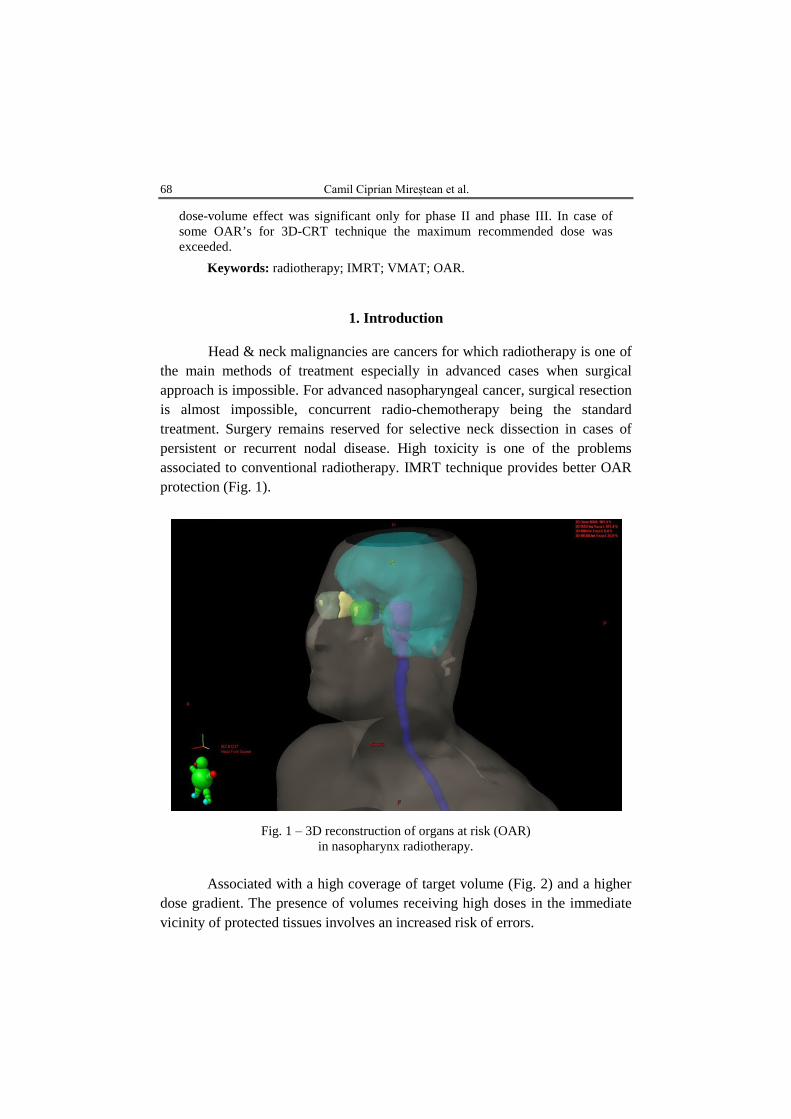
68 Camil Ciprian Mireștean et al.
dose-volume effect was significant only for phase II and phase III. In case of some OAR’s for 3D-CRT technique the maximum recommended dose was exceeded.
Keywords: radiotherapy; IMRT; VMAT; OAR.
1. Introduction Head & neck malignancies are cancers for which radiotherapy is one of
the main methods of treatment especially in advanced cases when surgical approach is impossible. For advanced nasopharyngeal cancer, surgical resection is almost impossible, concurrent radio-chemotherapy being the standard treatment. Surgery remains reserved for selective neck dissection in cases of persistent or recurrent nodal disease. High toxicity is one of the problems associated to conventional radiotherapy. IMRT technique provides better OAR protection (Fig. 1).
Fig. 1 ‒ 3D reconstruction of organs at risk (OAR) in nasopharynx radiotherapy.
Associated with a high coverage of target volume (Fig. 2) and a higher
dose gradient. The presence of volumes receiving high doses in the immediate vicinity of protected tissues involves an increased risk of errors.
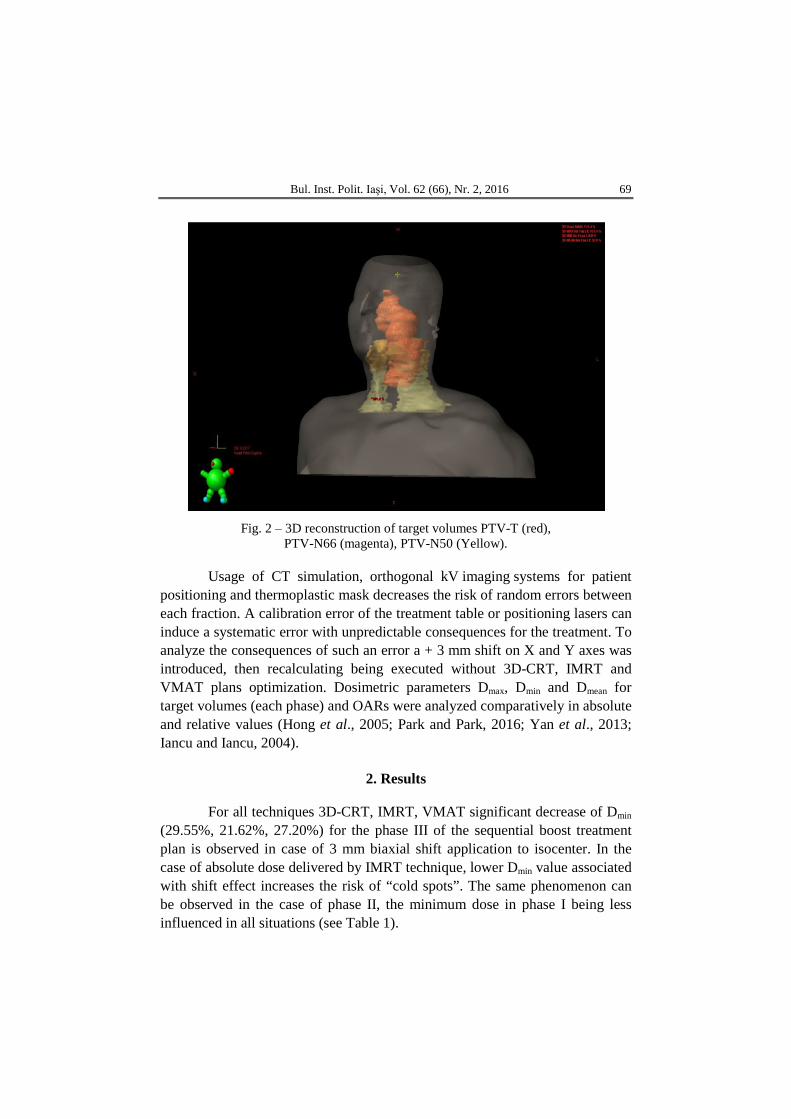
Bul. Inst. Polit. Iaşi, Vol. 62 (66), Nr. 2, 2016 69
Fig. 2 ‒ 3D reconstruction of target volumes PTV-T (red),
PTV-N66 (magenta), PTV-N50 (Yellow).
Usage of CT simulation, orthogonal kV imaging systems for patient positioning and thermoplastic mask decreases the risk of random errors between each fraction. A calibration error of the treatment table or positioning lasers can induce a systematic error with unpredictable consequences for the treatment. To analyze the consequences of such an error a + 3 mm shift on X and Y axes was introduced, then recalculating being executed without 3D-CRT, IMRT and VMAT plans optimization. Dosimetric parameters Dmax, Dmin and Dmean for target volumes (each phase) and OARs were analyzed comparatively in absolute and relative values (Hong et al., 2005; Park and Park, 2016; Yan et al., 2013; Iancu and Iancu, 2004).
2. Results
For all techniques 3D-CRT, IMRT, VMAT significant decrease of Dmin
(29.55%, 21.62%, 27.20%) for the phase III of the sequential boost treatment plan is observed in case of 3 mm biaxial shift application to isocenter. In the case of absolute dose delivered by IMRT technique, lower Dmin value associated with shift effect increases the risk of “cold spots”. The same phenomenon can be observed in the case of phase II, the minimum dose in phase I being less influenced in all situations (see Table 1).
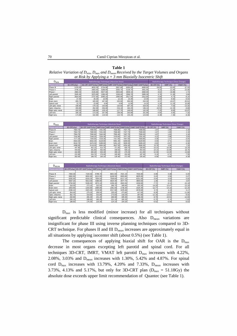
70 Camil Ciprian Mireștean et al.
Table 1 Relative Variation of Dmin, Dmax and Dmean Received by the Target Volumes and Organs
at Risk by Applying a + 3 mm Biaxially Isocentric Shift
Dmax is less modified (minor increase) for all techniques without
significant predictable clinical consequences. Also Dmean variations are insignificant for phase III using inverse planning techniques compared to 3D-CRT technique. For phases II and III Dmean increases are approximately equal in all situations by applying isocenter shift (about 0.5%) (see Table 1).
The consequences of applying biaxial shift for OAR is the Dmax decrease in most organs excepting left parotid and spinal cord. For all techniques 3D-CRT, IMRT, VMAT left parotid Dmax increases with 4.22%, 2.08%, 3.03% and Dmean increases with 1.30%, 5.42% and 4.87%. For spinal cord Dmax increases with 13.79%, 4.20% and 7.33%, Dmean increases with 3.73%, 4.13% and 5.17%, but only for 3D-CRT plan (Dmax = 51.18Gy) the absolute dose exceeds upper limit recommendation of Quantec (see Table 1).
DMINPhases and OARs 3D-CRT(cGy) 3D-CRT-SHIFT(cGy) IMRT(cGy) IMRT-SHIFT(cGy) VMAT(cGy) VMAT-SHIFT(cGy) 3D-CRT (%) IMRT (%) VMAT (%)Phase III 5725.00 4033.30 3734.90 2927.40 6295.20 4583.00 -29.55 -21.62 -27.20Phase II 3746.10 3400.40 3288.80 2583.70 5138.70 3931.90 -9.23 -21.44 -23.48Phase I 2860.20 3106.80 5927.00 4926.80 3008.10 3060.00 8.62 -16.88 1.73Left parotid 3345.40 3370.80 1390.40 1548.40 2589.70 2685.30 0.76 11.36 3.69Right parotid 2824.90 2737.60 2095.10 1995.90 2517.40 2312.60 -3.09 -4.73 -8.14Brain 27.30 26.20 13.00 12.10 15.30 14.30 -4.03 -6.92 -6.54Brain stem 200.70 183.90 167.80 150.90 264.90 210.30 -8.37 -10.07 -20.61Spinal cord 22.70 23.90 8.90 9.90 12.90 14.20 5.29 11.24 10.08Left optic nerve 190.90 179.10 144.80 134.60 367.20 318.20 -6.18 -7.04 -13.34Optic chiasma 293.80 262.90 246.00 216.10 160.20 146.10 -10.52 -12.15 -8.80Right optic nerve 182.00 168.80 129.10 117.70 148.60 132.30 -7.25 -8.83 -10.97Left lens 184.10 173.20 147.00 138.30 163.90 151.90 -5.92 -5.92 -7.32Right lens 173.90 162.80 119.50 110.70 135.20 123.90 -6.38 -7.36 -8.36
Radiotherapy Technique (Absolute Dose) Radiotherapy Technique (Dose Change)
DMAXPhases and OARs 3D-CRT(cGy) 3D-CRT-SHIFT(cGy) IMRT(cGy) IMRT-SHIFT(cGy) VMAT(cGy) VMAT-SHIFT(cGy) 3D-CRT (%) IMRT (%) VMAT (%)Phase III 7564.70 7690.90 7441.00 7566.80 7427.70 7590.00 1.67 1.69 2.19Phase II 7564.70 7690.90 7441.00 7566.80 7427.70 7590.00 1.67 1.69 2.19Phase I 7564.70 7690.90 7416.90 7560.40 7427.70 7590.00 1.67 1.93 2.19Left parotid 7242.80 7548.20 7326.30 7478.60 7077.20 7291.50 4.22 2.08 3.03Right parotid 7177.20 7205.00 7218.30 7317.00 7047.60 7009.80 0.39 1.37 -0.54Brain 6919.20 6642.30 6128.80 5901.40 6269.60 6229.90 -4.00 -3.71 -0.63Brain stem 6518.70 6476.30 5498.80 5451.10 5609.30 5589.20 -0.65 -0.87 -0.36Spinal cord 4498.00 5118.20 4364.40 4547.50 4254.40 4566.30 13.79 4.20 7.33Left optic nerve 447.90 402.10 414.70 371.60 600.70 538.90 -10.23 -10.39 -10.29Optic chiasma 444.60 381.80 402.90 338.60 509.10 454.30 -14.13 -15.96 -10.76Right optic nerve 416.90 365.40 333.40 289.10 476.20 411.00 -12.35 -13.29 -13.69Left lens 215.90 204.70 176.00 165.90 202.60 187.30 -5.19 -5.74 -7.55Right lens 202.00 188.70 145.10 135.40 171.50 155.40 -6.58 -6.69 -9.39
Radiotherapy Technique (Absolute Dose) Radiotherapy Technique (Dose Change)
DMEANPhases and OARs 3D-CRT(cGy) 3D-CRT-SHIFT(cGy) IMRT(cGy) IMRT-SHIFT(cGy) VMAT(cGy) VMAT-SHIFT(cGy) 3D-CRT (%) IMRT (%) VMAT (%)
Phase III 7094.30 7100.50 6798.70 6831.00 7021.10 7034.80 0.09 0.48 0.20Phase II 6902.90 6932.60 6213.90 6248.50 6803.80 6835.80 0.43 0.56 0.47Phase I 6282.00 6316.20 7004.50 7039.60 6217.10 6251.50 0.54 0.50 0.55Left parotid 5837.20 5913.00 4386.80 4624.40 4577.70 4800.60 1.30 5.42 4.87Right parotid 5794.90 5348.40 4573.10 4156.40 4943.30 4439.80 -7.71 -9.11 -10.19Brain 318.30 273.10 315.50 266.70 349.40 303.30 -14.20 -15.47 -13.19Brain stem 1654.90 1443.60 1585.80 1361.50 1736.30 1525.30 -12.77 -14.14 -12.15Spinal cord 2336.10 2423.30 2129.90 2217.90 1976.40 2078.60 3.73 4.13 5.17Left optic nerve 304.40 279.20 258.50 235.00 473.80 417.60 -8.28 -9.09 -11.86Optic chiasma 362.70 318.60 315.80 273.00 318.20 287.80 -12.16 -13.55 -9.55Right optic nerve 294.90 266.30 231.20 206.90 305.00 268.40 -9.70 -10.51 -12.00Left lens 200.10 188.60 160.30 151.10 182.20 168.30 -5.75 -5.74 -7.63Right lens 188.60 176.30 133.30 124.10 154.20 140.90 -6.52 -6.90 -8.63
Radiotherapy Technique (Absolute Dose) Radiotherapy Technique (Dose Change)
Bul. Inst. Polit. Iaşi, Vol. 62 (66), Nr. 2, 2016 71
3. Discussion
The use of modern radiotherapy methods has reduced the volume
exposed to large doses of radiation therapy, improving treatment accuracy, reducing normal tissue toxicity related to irradiation, increased importance given to accurate position verification and correction before delivering radiotherapy. IGRT enables evaluation of geometry for treatment delivery providing a method by which deviations from the original plan of anatomy are determined and this information is used to correct the dosimetric parameters. Bony landmarks were easy to detect and correct and the table shifts for correction of setup deviations could be automatically calculated. An error in radiotherapy is any deviation from intended or planned treatment (Hong et al., 2005; Thilmann et al., 2006; Dawson and Jaffray, 2007).
The risk of a systematic error is low but the clinical consequences can be unpredictable if the error is not corrected before or during treatment. Decrease of Dmin in phase III corresponds to target volumes that will receive the entire dose of 70Gy/35 fractions increases the number of cold spots associated with risk of under-dosage in primary tumor volume. The association between a Dmin decreased in absolute and relative decrease of Dmin by applying “simulated error”, the presence of “cold spots” in a radio-resistant hypoxic zone may be a factor associated with the presence of a residual tumor at the end of treatment. In this case IMRT technique is associated with a higher risk of under-dosage for target volume of primary tumors of the nasopharynx than 3D-CRT and VMAT techniques. By applying the biaxial isocenter shift laterocervical nodal levels (PTV-N66) shows a lower risk of under-dosage than (PTV-T) and the dose effect to supraclavicular nodal (PTV-N50) level is insignificant (Fig. 2). The presence of clinically detectable lymph nodes with a good response to therapy or a significant patient weight loss resulting in neck circumference reduction associated with isocentric shift can bring the skin in the build-up dose area, especially for the case of IMRT technique with more tangential fields (Iancu and Iancu, 2004; Kaur et al., 2016; Liu et al., 2016).
4. Conclusions
A systematic error of + 3 mm biaxial shift applied to isocenter has no
severe consequences on the quality of treatment of nasopharyngeal primary tumor but may result in under-dosage in laterocervical nodal volumes. Adding a random error to the induced systematic error can amplify or reduce the dosimetric effects. In the case of exceeding the value of the total error beyond
72 Camil Ciprian Mireștean et al.
the distance limit that manifests intense dose gradient for IMRT and VMAT methods there is a major possibility to irradiation with major dosimetric consequences for the target volumes and normal tissue. Immobilization systems (thermoplastic masks), IG systems and an accurate calibration of the treatment table and positioning lasers ensure the quality of treatment.
REFERENCES Dawson L.A., Jaffray D.A., Advances in Image-Guided Radiation Therapy, Journal of
Clinical Oncology, 25, 8, 938-946 (2007). Hong T.S., Tomé W.A., Chappell R.J. et al., The Impact of Daily Setup Variations on
Head-and-Neck Intensity-Modulated Radiation Therapy, Int. J. Radiat. Oncol. Biol. Phys., 61, 3, 779-788 (2005).
Iancu D.T, Iancu R.I., Use of Simulator in Treatment Planning and Determination and Definition of Treatment Volume, Rev. Med. Chir. Soc. Med. Nat. Iași, 108, 3, 580-583 (2004).
Kaur I., Rawat S., Ahlawat P. et al., Dosimetric Impact of Setup Errors in Head and Neck Cancer Patients Treated by Image-Guided Radiotherapy, J. Med. Phys., 41, 2, 144-148 (2016).
Liu G., Zhang S., Ma Y. et al., Effects of Error on Dose of Target Region and Organs at Risk in Treating Nasopharynx Cancer with Intensity Modulated Radiation Therapy, Pak. J. Med. Sci., 32, 1, 95-100 (2016).
Park E.T., Park S.K., Setup Uncertainties for Inter-Fractional Head and Neck Cancer in Radiotherapy, Oncotarget, 2016, May 31, doi: 10.18632/oncotarget.9748.
Thilmann C., Nill S., Tücking T. et al., Correction of Patient Positioning Errors Based on In-Line Cone Beam CTs: Clinical Implementation and First Experiences. Radiat. Oncol., 1:16 (2006).
Yan M., Lovelock D., Hunt M. et al., Measuring Uncertainty in Dose Delivered to the Cochlea Due to Setup Error During External Beam Treatment of Patients with Cancer of the Head and Neck, Med. Phys. (2013).
EFECTUL DOZIMETRIC AL ERORILOR SISTEMATICE DE POZIȚIONARE PRIN INDUCEREA ARTIFICIALĂ A UNEI DEPLASĂRI BIAXIALE
DE 3 mm A MESEI DE TRATAMENT ÎN RADIOTERAPIA EXTERNĂ A CANCERULUI DE RINOFARINGE LOCAL AVANSAT
(Rezumat)
Cancerele sferei ORL sunt patologii în care radioterapia este de multe ori
metoda principală de tratament, în special în cazurile avansate, depășite chirurgical. Analizăm efectul dozimetric a unei deplasări biaxile, de 3 mm, asupra izocentrului, aplicând un shift pe axele x și y de + 3 mm și evaluând dozele la organele de risc și în volumele țintă PTV-T (volumul țintă al tumorii primare), care a primit o doză de 70Gy
Bul. Inst. Polit. Iaşi, Vol. 62 (66), Nr. 2, 2016 73
în 35 fracțiuni (faza I), PTV- N66 (faza II) și PTV-N50 (faza III) pentru ariile gaglionare laterocervicale și supraclaviculare iradiate cu 66, respectiv 50Gy în 33 și 25 fracțiuni, prin tehnica boost-ului secvențial. Evaluarea parametrilor dozimetrici Dmax, Dmean și Dmin s-a făcut atât pentru volumele țintă cât și pentru OAR (organele de risc) înainte și după aplicarea shiftului pentru planurile 3D-CRT (3D conformațional) și pe planurile alternative IMRT (radioterapie cu intensitate modulată) și VMAT (radioterapie rotațională cu intensitate modulată). Efectul asupra volumelor țintă ca distribuție a dozei a fost semnificativ doar în fazele II și III. În cazul OAR, prin tehnica 3D, în urma shiftului s-a depășit doza maximă recomandată de ghidul dozimetric QUANTEC.
