mixing process in rotating motions · 2010-08-25 · mixing process in rotating motions 197 the...

U.P.B. Sci. Bull., Series D, Vol. 72, Iss. 2, 2010 ISSN 1454-2358

MIXING PROCESS IN ROTATING MOTIONS

Cătălin MĂRCULESCU1, Corneliu BĂLAN2

Lucrarea este dedicată investigaţiilor procesului de amestec generat de un rotor in mişcare de rotaţie, în interiorul unui vas cilindric. Studiul îşi propune o comparaţie a rezultatelor experimentale cu predicţiile numerice pentru mişcarea de rotaţie a discului, a elicei si a unui ansamblu de elice în incinte închise, având ca obiective: (i) validarea codului numeric FLUENT in configuraţii test (disc), având la baza şi studii teoretice din literatura de specialitate; (ii) stabilirea unor proceduri numerice pentru simularea hidrodinamicii amestecătorului; (iii) determinarea unei modalităţi de cuantificare a gradului de amestec utilizând diverse configuraţii ale amestecătorului (camera de amestec + rotor). Lucrarea evidenţiază buna corelare intre experiment si predicţiile numerice si importanta deosebită pentru validarea codului numeric în aplicaţiile tehnice prin tehnici de vizualizare si măsurare a presiunii.

The paper is concerned with the investigations of the mixing process generated by a spinning rotor inside an enclosed cylindrical vessel. The aim of the study is to compare experimental results with numerical predictions for a rotating disk and an impeller with the following leading objectives: (i) FLUENT code validation using test configurations (disk), with links to the theoretical studies in the literature; (ii) development of numerical procedures for the hydrodynamics simulation of a chemical reactor; (iii) determination of quantifying methods for the mixing degree using alternative configurations of the reactor (mixing chamber + rotor). The work emphasizes a good correlation between experiments and computation and also the importance in applied hydrodynamics of numerical code validation through visualizations techniques and pressure measurements.

Keywords: flow visualizations; numerical simulations; laminar flows; rotational motions; vorticity number; mixing coefficient.

1. Introduction

The mixing process dynamics is determined by the pressure gradients generated inside a vessel by a spinning rotor. This principle applies no matter the shape of the generating rotor. It can be a simple rotating cylinder (Taylor-Couette motion [1]), a disk, an impeller or a structure of impellers. The notable difference between the shapes is given by the efficiency of transformation of mechanical energy into kinetic energy and by the mixing degree inside the vessel [2]. 1 PhD student, Dept. of Hydraulics, University POLITEHNICA of Bucharest, Romania, e-mail: [email protected]; 2 Professor, Dept. of Hydraulics, University POLITEHNICA of Bucharest, Romania

196 Cătălin Mărculescu, Corneliu Bălan

The aim of the study is to compare experimental results with numerical predictions for a rotating disk and an impeller in closed vessels, with the following leading objectives: (i) FLUENT numerical code validation using test configurations (disk), with links to the theoretical studies in the literature; (ii) development of numerical procedures for the hydrodynamics simulation of a chemical reactor; (iii) determination of quantifying methods for the mixing degree using alternative configurations of the reactor (mixing chamber + rotor). The influences of mixing degree on product composition have been investigated for reactors and mixers of macro- [3] and micro-scales [4]. Several studies approached this issue by using computational fluid dynamics (CFD) [5, 6].

Numerical simulations and the experimental investigations are performed in a laminar flow regime, isothermal conditions, with 1000 as the maximum value for Reynolds number (Re = ρωR2/η0).

Working fluids are incompressible Newtonian fluids with η = 0.001÷1Pa·s.

1.1 Evolution of the working geometry

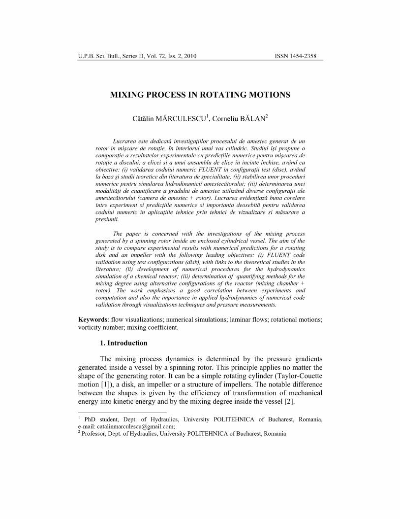
The investigations were initialized by a test case found in the theoretical studies from the literature: spinning disk in an enclosed cylindrical vessel (Fig. 1).

This test case is used to validate the numerical code, FLUENT with the

pre-processor GAMBIT, for the simulation and representation of rotational motions, geometry generations and discretizing flow domains. FLUENT is using C computer language for its flexibility and power, obtaining a real time allocation of the dynamic memory, efficient data structures and flexible solver control [7].

Fig. 1. 3D model of the mixing chamber with a spinning disk; 2D slice of the mesh: h1 = 19 mm; h2 = 40 mm; d1 = 10 mm; d2 = 40 mm; d3 = 50 mm; δ = 2 mm.

d2

d3

Static walls h1

d1Rotating disk

h2 δ

Mixing process in rotating motions 197

The flow domain has been split into 119226 hexahedral finite elements (cells), using a Cooper mesh generation scheme. The scheme sweeps the mesh node patterns of specified "source" faces through the volume. In this case, without a high complexity and with axial symmetry, it was possible to generate a structured mesh, without introducing a high number of cells.

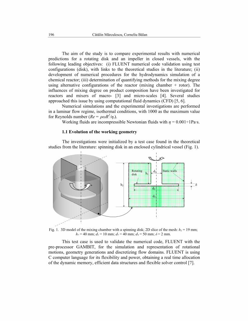
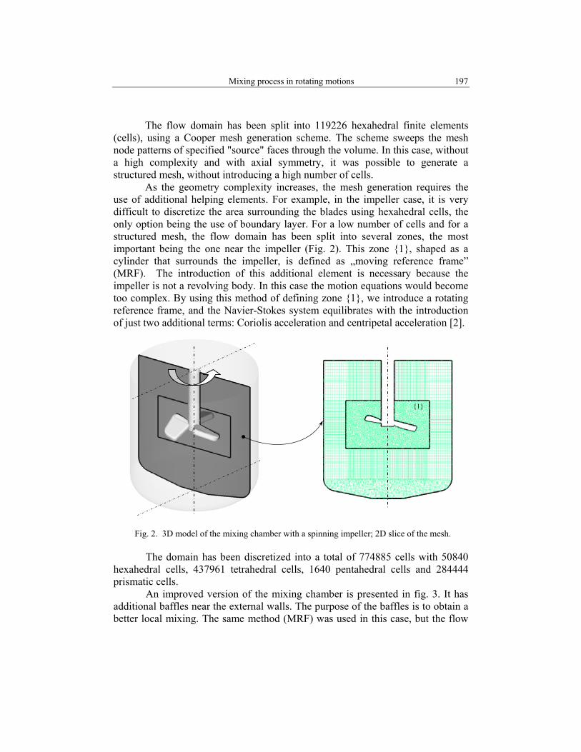
As the geometry complexity increases, the mesh generation requires the use of additional helping elements. For example, in the impeller case, it is very difficult to discretize the area surrounding the blades using hexahedral cells, the only option being the use of boundary layer. For a low number of cells and for a structured mesh, the flow domain has been split into several zones, the most important being the one near the impeller (Fig. 2). This zone 1, shaped as a cylinder that surrounds the impeller, is defined as „moving reference frame” (MRF). The introduction of this additional element is necessary because the impeller is not a revolving body. In this case the motion equations would become too complex. By using this method of defining zone 1, we introduce a rotating reference frame, and the Navier-Stokes system equilibrates with the introduction of just two additional terms: Coriolis acceleration and centripetal acceleration [2]. The domain has been discretized into a total of 774885 cells with 50840 hexahedral cells, 437961 tetrahedral cells, 1640 pentahedral cells and 284444 prismatic cells. An improved version of the mixing chamber is presented in fig. 3. It has additional baffles near the external walls. The purpose of the baffles is to obtain a better local mixing. The same method (MRF) was used in this case, but the flow

Fig. 2. 3D model of the mixing chamber with a spinning impeller; 2D slice of the mesh.

1


domain has been discretized using only tetrahedral cells, with a higher mesh refinement than the previous case: 1273857 cells. This is the configuration of the chemical reactor for polymerization used in the investigations of flow optimization. The aim of these investigations is the homogenization of the final compounds, resulting from the polymerization process.

1.2. Vorticity number

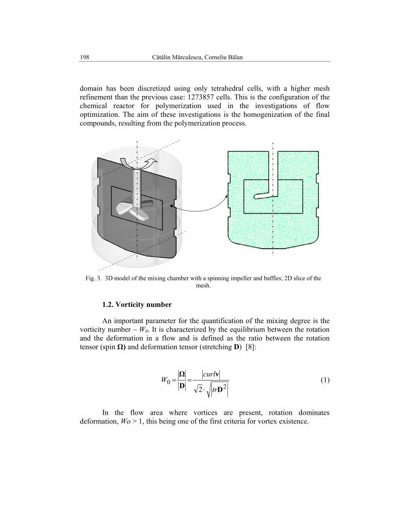
An important parameter for the quantification of the mixing degree is the vorticity number – W0. It is characterized by the equilibrium between the rotation and the deformation in a flow and is defined as the ratio between the rotation tensor (spin Ω) and deformation tensor (stretching D) [8]:

20

2 D

vDΩ

tr

curlW

⋅== (1)

In the flow area where vortices are present, rotation dominates

deformation, Wo > 1, this being one of the first criteria for vortex existence.

Fig. 3. 3D model of the mixing chamber with a spinning impeller and baffles; 2D slice of the mesh.


2. Experiment

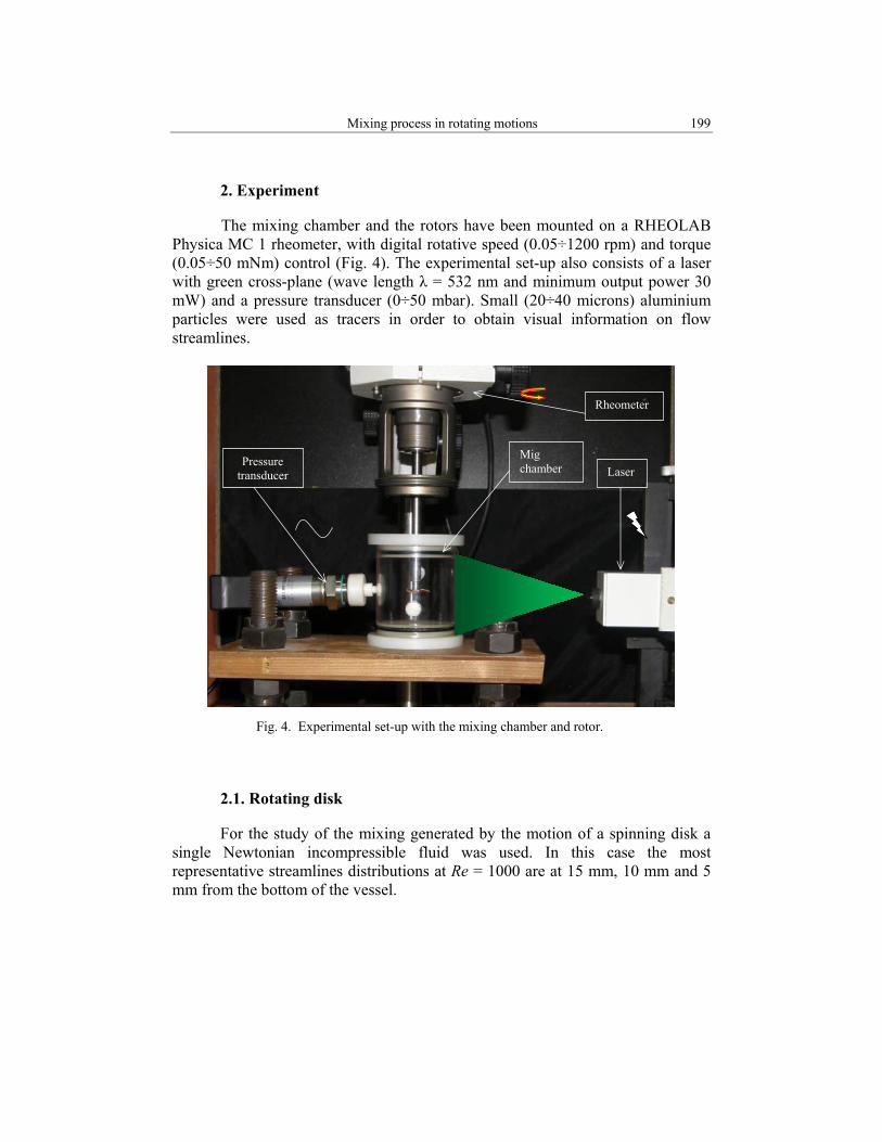
The mixing chamber and the rotors have been mounted on a RHEOLAB Physica MC 1 rheometer, with digital rotative speed (0.05÷1200 rpm) and torque (0.05÷50 mNm) control (Fig. 4). The experimental set-up also consists of a laser with green cross-plane (wave length λ = 532 nm and minimum output power 30 mW) and a pressure transducer (0÷50 mbar). Small (20÷40 microns) aluminium particles were used as tracers in order to obtain visual information on flow streamlines.

2.1. Rotating disk

For the study of the mixing generated by the motion of a spinning disk a single Newtonian incompressible fluid was used. In this case the most representative streamlines distributions at Re = 1000 are at 15 mm, 10 mm and 5 mm from the bottom of the vessel.

Rheometer

Laser Mig chamber Pressure

transducer

Fig. 4. Experimental set-up with the mixing chamber and rotor.


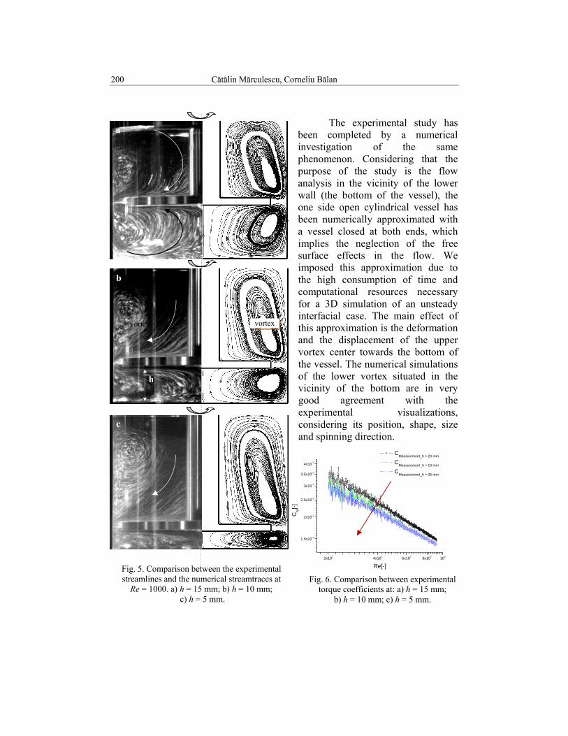
Fig. 5. Comparison between the experimental streamlines and the numerical streamtraces at

Re = 1000. a) h = 15 mm; b) h = 10 mm; c) h = 5 mm.

2x102 4x102 6x102 8x102 103

1.5x10-1

2x10-1

2.5x10-1

3x10-1

3.5x10-1

4x10-1

CM[-]

Re[-]

CMeasurement_h = 20 mm



a

b

c

h

vortex vortex

The experimental study has been completed by a numerical investigation of the same phenomenon. Considering that the purpose of the study is the flow analysis in the vicinity of the lower wall (the bottom of the vessel), the one side open cylindrical vessel has been numerically approximated with a vessel closed at both ends, which implies the neglection of the free surface effects in the flow. We imposed this approximation due to the high consumption of time and computational resources necessary for a 3D simulation of an unsteady interfacial case. The main effect of this approximation is the deformation and the displacement of the upper vortex center towards the bottom of the vessel. The numerical simulations of the lower vortex situated in the vicinity of the bottom are in very good agreement with the experimental visualizations, considering its position, shape, size and spinning direction.

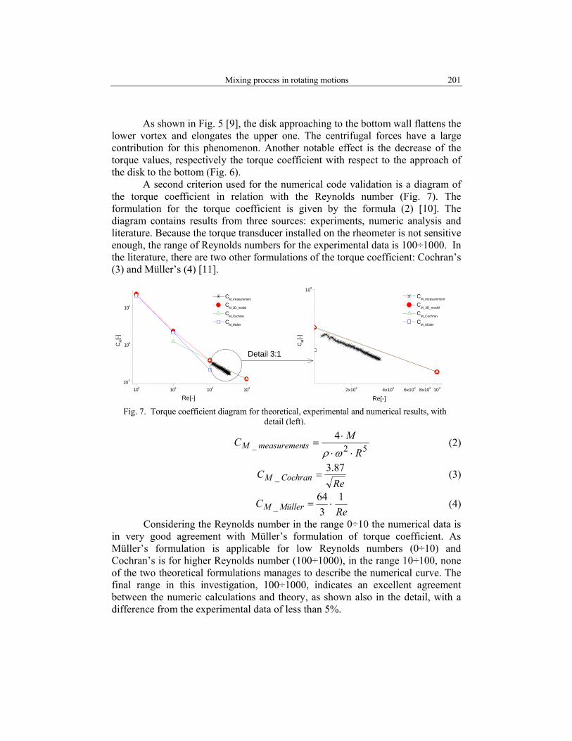
Fig. 6. Comparison between experimental

torque coefficients at: a) h = 15 mm; b) h = 10 mm; c) h = 5 mm.


As shown in Fig. 5 [9], the disk approaching to the bottom wall flattens the lower vortex and elongates the upper one. The centrifugal forces have a large contribution for this phenomenon. Another notable effect is the decrease of the torque values, respectively the torque coefficient with respect to the approach of the disk to the bottom (Fig. 6).

A second criterion used for the numerical code validation is a diagram of the torque coefficient in relation with the Reynolds number (Fig. 7). The formulation for the torque coefficient is given by the formula (2) [10]. The diagram contains results from three sources: experiments, numeric analysis and literature. Because the torque transducer installed on the rheometer is not sensitive enough, the range of Reynolds numbers for the experimental data is 100÷1000. In the literature, there are two other formulations of the torque coefficient: Cochran’s (3) and Müller’s (4) [11].

52_4

RMC tsmeasuremenM⋅⋅

⋅=

ωρ (2)

Re

C CochranM87.3

_ = (3)

Re

C MüllerM1

364

_ ⋅= (4)

Considering the Reynolds number in the range 0÷10 the numerical data is in very good agreement with Müller’s formulation of torque coefficient. As Müller’s formulation is applicable for low Reynolds numbers (0÷10) and Cochran’s is for higher Reynolds number (100÷1000), in the range 10÷100, none of the two theoretical formulations manages to describe the numerical curve. The final range in this investigation, 100÷1000, indicates an excellent agreement between the numeric calculations and theory, as shown also in the detail, with a difference from the experimental data of less than 5%.

Fig. 7. Torque coefficient diagram for theoretical, experimental and numerical results, with detail (left).

Re[-] Re[-] 100 101 102 103

10-1

100

101

CM[-]

CM_measurement

CM_3D_model

CM_Cochran

CM_Müller

2x102 4x102 6x102 8x102 103

100

CM[-]

CM_measurement

CM_3D_model

CM_Cochran

CM_Müller

Detail 3:1


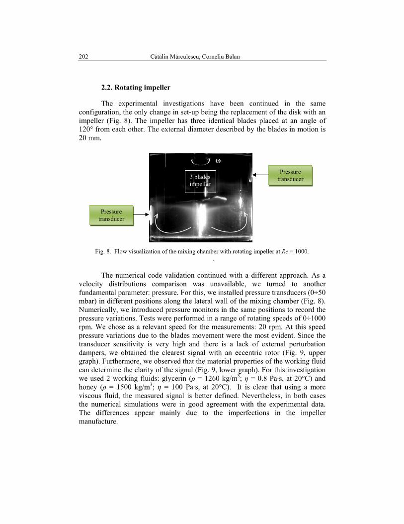
2.2. Rotating impeller

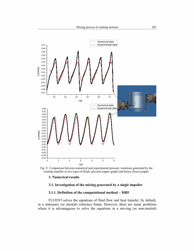
The experimental investigations have been continued in the same configuration, the only change in set-up being the replacement of the disk with an impeller (Fig. 8). The impeller has three identical blades placed at an angle of 120° from each other. The external diameter described by the blades in motion is 20 mm. The numerical code validation continued with a different approach. As a velocity distributions comparison was unavailable, we turned to another fundamental parameter: pressure. For this, we installed pressure transducers (0÷50 mbar) in different positions along the lateral wall of the mixing chamber (Fig. 8). Numerically, we introduced pressure monitors in the same positions to record the pressure variations. Tests were performed in a range of rotating speeds of 0÷1000 rpm. We chose as a relevant speed for the measurements: 20 rpm. At this speed pressure variations due to the blades movement were the most evident. Since the transducer sensitivity is very high and there is a lack of external perturbation dampers, we obtained the clearest signal with an eccentric rotor (Fig. 9, upper graph). Furthermore, we observed that the material properties of the working fluid can determine the clarity of the signal (Fig. 9, lower graph). For this investigation we used 2 working fluids: glycerin (ρ = 1260 kg/m3; η = 0.8 Pa·s, at 20°C) and honey (ρ = 1500 kg/m3; η = 100 Pa·s, at 20°C). It is clear that using a more viscous fluid, the measured signal is better defined. Nevertheless, in both cases the numerical simulations were in good agreement with the experimental data. The differences appear mainly due to the imperfections in the impeller manufacture.

Fig. 8. Flow visualization of the mixing chamber with rotating impeller at Re = 1000. .

Pressure transducer

Pressure transducer 3 blades

impeller

ω


3. Numerical results

3.1. Investigation of the mixing generated by a single impeller

3.1.1. Definition of the computational method – MRF

FLUENT solves the equations of fluid flow and heat transfer, by default, in a stationary (or inertial) reference frame. However, there are many problems where it is advantageous to solve the equations in a moving (or non-inertial)

Fig. 9. Comparison between numerical and experimental pressure variations generated by the rotating impeller in two types of fluids: glycerin (upper graph) and honey (lower graph).

0 1 2 3 4 5 6-0.10-0.09-0.08-0.07-0.06-0.05-0.04-0.03-0.02-0.010.000.010.020.030.040.050.060.070.08

p [m

bar]

t [s]

Numerical data Experimental data

22 23 24 25 26 27

-0.07

-0.06

-0.05

-0.04

-0.03

-0.02

-0.01

0.00

0.01

0.02

0.03

0.04

0.05

0.06

0.07

p [m

bar]

t [s]

Numerical data Experimental data


reference frame. Such problems typically involve moving parts (such as rotating blades, impellers, and similar types of moving surfaces), and it is the flow around these moving parts that is of interest. In most cases, the moving parts render the problem unsteady when viewed from the stationary frame. With a moving reference frame, however, the flow around the moving part can (with certain restrictions) be modeled as a steady-state problem with respect to the moving frame.

FLUENT's moving reference frame modeling capability allows to model problems involving moving parts by activating moving reference frames in selected cell zones. When a moving reference frame is activated, the equations of motion are modified to incorporate the additional acceleration terms which occur due to the transformation from the stationary to the moving reference frame. By solving these equations in a steady-state manner, the flow around the moving parts can be modeled.

For simple problems, it may be possible to refer the entire computational domain to a single moving reference frame. This is known as the single reference frame approach - SRF. The use of the SRF approach is possible, provided the geometry meets certain requirements. For more complex geometries, it may not be possible to use a single reference frame. In such cases, you must break up the problem into multiple cells zones, with well-defined interfaces between the zones. The manner in which the interfaces are treated leads to two approximate, steady-state modeling methods for this class of problem: the multiple reference frame approach, and the mixing plane approach. If unsteady interaction between the stationary and moving parts is important, one can employ the Sliding Mesh approach to capture the transient behavior of the flow.

For a steady rotating frame (the rotational speed is constant), it is possible to transform the equations of fluid motion to the rotating frame such that steady-state solutions are possible. By default, FLUENT permits the activation of a moving reference frame with a steady rotational speed. If the rotational speed is not constant, the transformed equations will contain additional terms which are not included in FLUENT's formulation (although they can be added as source terms using user-defined functions). Also it should be noted that one can run an unsteady simulation in a moving reference frame with constant rotational speed. This would be necessary if one wants to simulate, for example, vortex shedding from a rotating fan blade. The unsteadiness in this case is due to a natural fluid instability (vortex generation) rather than induced from interaction with a stationary component [7].


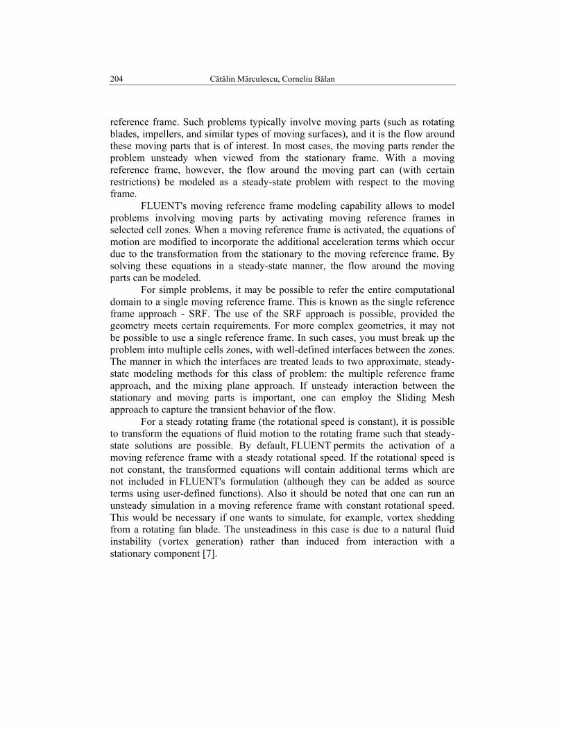
3.1.2. Simulation of the mixing process

To emphasize the importance of MRF (Moving Reference Frame) in the computational scheme, we performed simulations of identical cases, the only difference being the condition of MRF. We compared the two cases with respect to pressure and velocity distributions, streamtraces, vorticity number, wall shear stress and pressure distributions (Figs. 10, 11, 12, 13).

The differences between the solutions are significant. As shown in all distributions, the case without MRF fails to properly describe the physical phenomenon. The most obvious differences are in the streamtraces distribution

Fig. 10. a) Pressure distributions at Re = 1000 without MRF (left) and with MRF (right); b) Velocity distributions at Re = 1000 without MRF (left) and with MRF (right).

a

b

p = ct

v = ct


a

b

W0 = 1

W0 > 1

W0 < 1

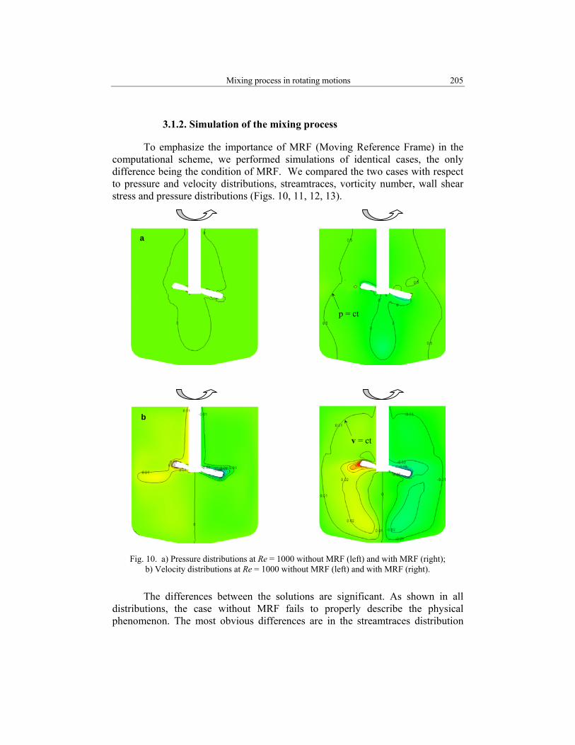
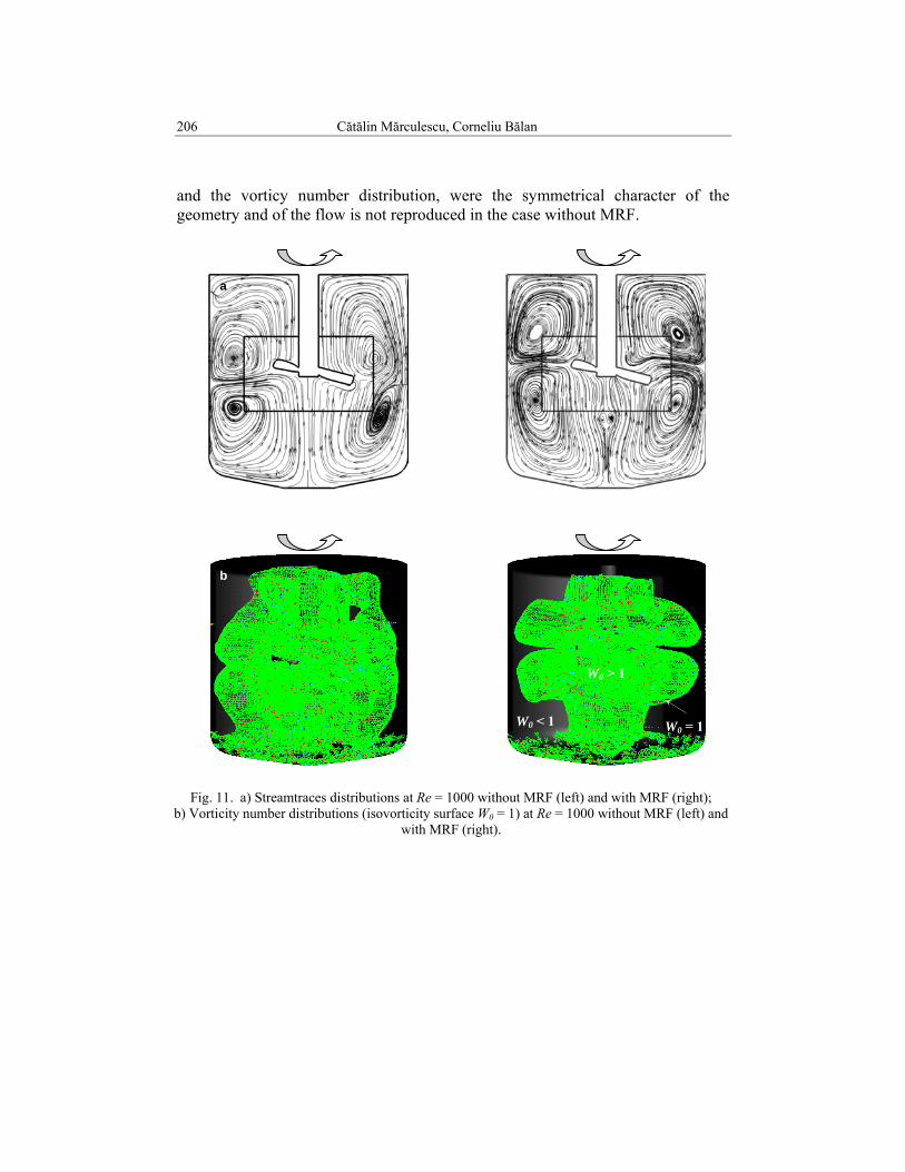
and the vorticy number distribution, were the symmetrical character of the geometry and of the flow is not reproduced in the case without MRF.

Fig. 11. a) Streamtraces distributions at Re = 1000 without MRF (left) and with MRF (right); b) Vorticity number distributions (isovorticity surface W0 = 1) at Re = 1000 without MRF (left) and

with MRF (right).


2:1 b

2:1 a

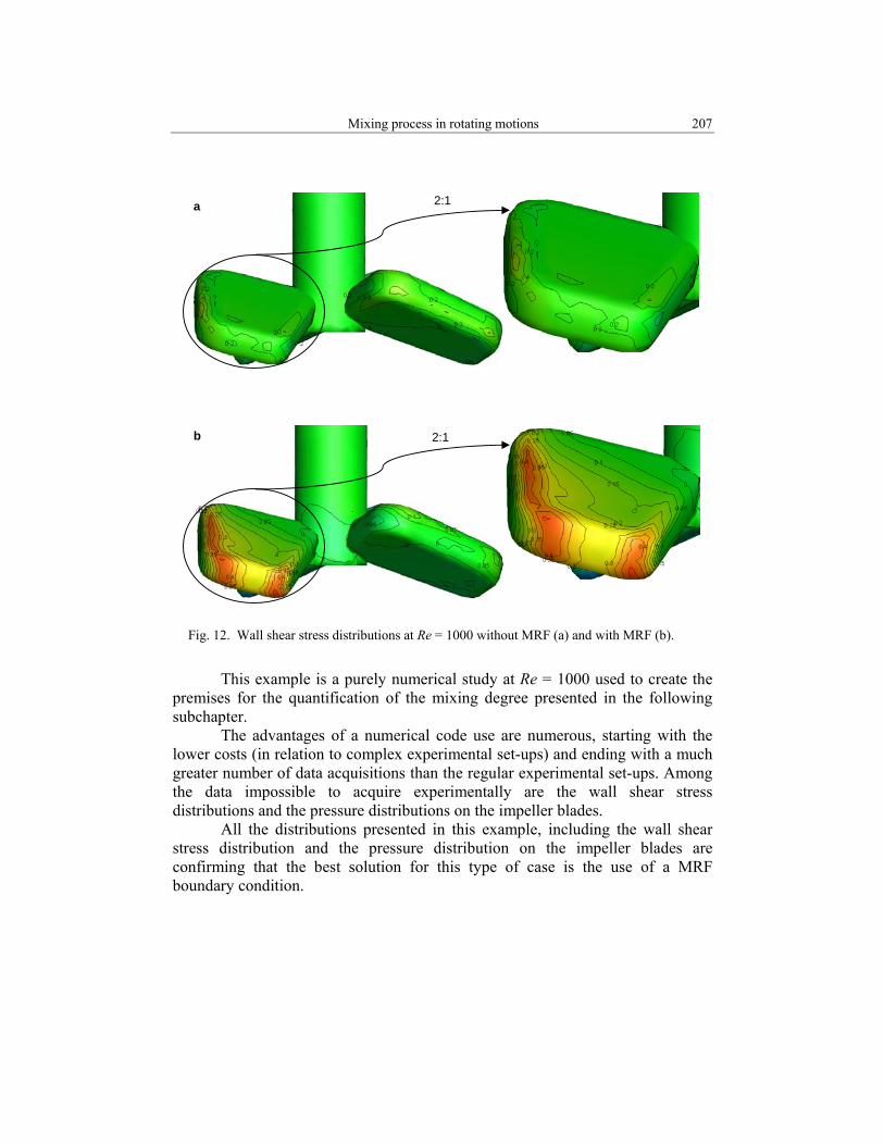
This example is a purely numerical study at Re = 1000 used to create the premises for the quantification of the mixing degree presented in the following subchapter. The advantages of a numerical code use are numerous, starting with the lower costs (in relation to complex experimental set-ups) and ending with a much greater number of data acquisitions than the regular experimental set-ups. Among the data impossible to acquire experimentally are the wall shear stress distributions and the pressure distributions on the impeller blades. All the distributions presented in this example, including the wall shear stress distribution and the pressure distribution on the impeller blades are confirming that the best solution for this type of case is the use of a MRF boundary condition.

Fig. 12. Wall shear stress distributions at Re = 1000 without MRF (a) and with MRF (b).


2:1 b

2:1 a

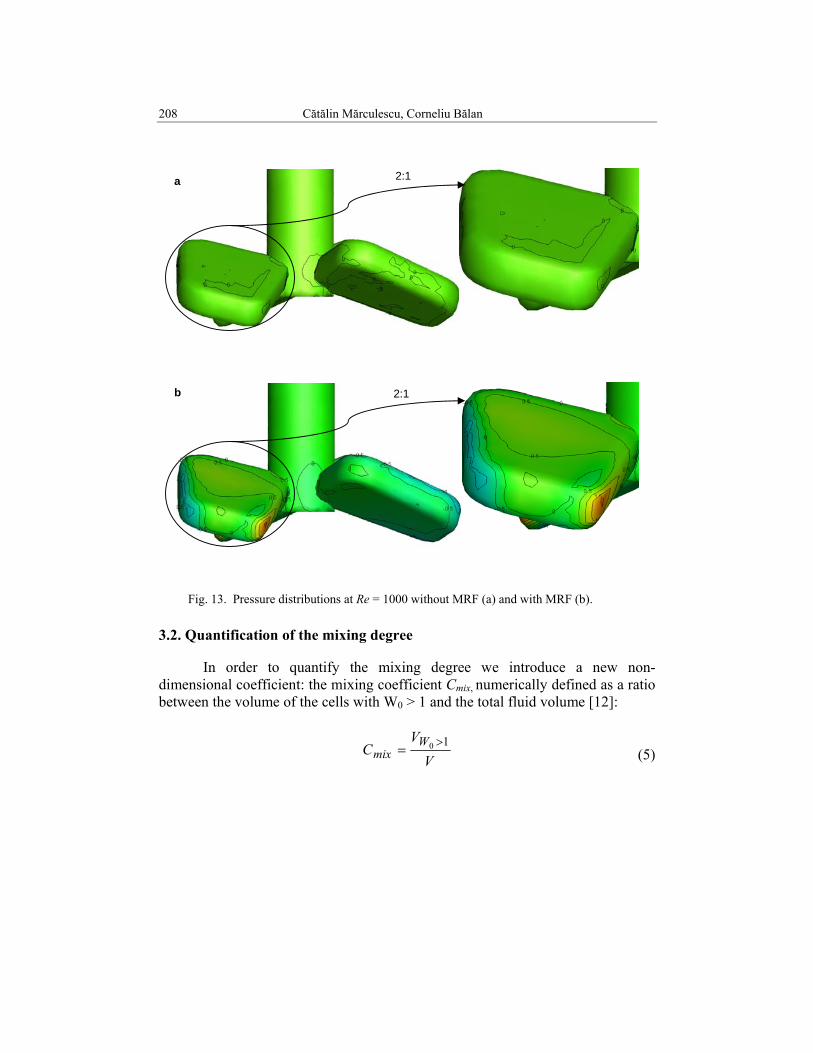
3.2. Quantification of the mixing degree

In order to quantify the mixing degree we introduce a new non-dimensional coefficient: the mixing coefficient Cmix, numerically defined as a ratio between the volume of the cells with W0 > 1 and the total fluid volume [12]:

(5)

Fig. 13. Pressure distributions at Re = 1000 without MRF (a) and with MRF (b).

VV

C Wmix

10 >=


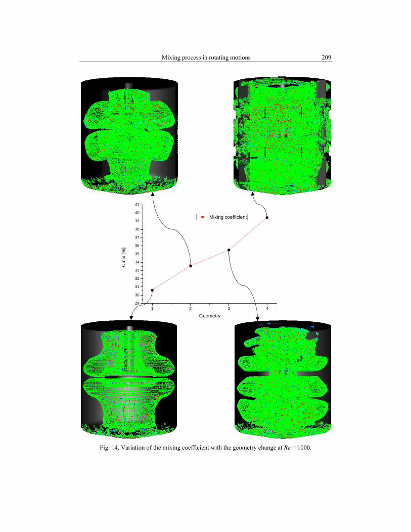
Fig. 14. Variation of the mixing coefficient with the geometry change at Re = 1000.

1 2 3 429

30

31

32

33

34

35

36

37

38

39

40

41

Cm

ix [%

]

Geometry

Mixing coefficient


In order to emphasize the influence of the geometry on the mixing degree, we consider four configurations to test the applicability of the mixing coefficient. In Fig. 14 the vorticity number distributions are represented for: i) a mixing chamber with a disk (geom. 1); ii) a mixing chamber with one impeller (geom. 2); iii) a mixing chamber with two impellers (geom. 3); iv) a mixing chamber with two impellers and baffles on the side walls (geom. 4). The values obtained for the mixing coefficient (table 1) have been corroborated with the vorticity number distributions to accentuate the increase of the mixing degree with the evolution of the working geometry.

Table 1 Values for the mixing coefficient

4. Final remarks

The main objective of this study, (i.e.) validation of the numerical code FLUENT, has been successfully achieved both in the spinning disk test case and the cases with impellers as mixing geometries. The validation has been performed in the range Re = 0÷1000 (in the laminar flow regime). Qualitatively and quantitatively, the numerical predictions matched the experimental and theoretical results. The next step in our research was to establish a numerical procedure to make precise predictions of the flow inside the polymerization reactor’s mixing chamber [13]. Determination of the proper geometry and mesh generation, the solver, the boundary conditions and the computational methods are essential in this research. We established a criteria for mixing, namely the mixing coefficient Cmix which can be used to distinguish between different working conditions and impeller designs. The final aim of the research is the optimization of the flow in the mixing chamber of the chemical reactor for polymerization. The process of modeling of the polymerization process will be an important part of the research.

5. Acknowledgements

The present work has been supported by the Romanian National Research Council – CNCSIS: research grant RU-TD-383. The experimental and numerical investigations have been performed in the REOROM Laboratory, University

Mixing geometry %CmixDisk 30.60 1 impeller 33.58 2 impellers 35.49 2 impellers + baffles 39.44


“Politehnica” of Bucharest and in the Multimaterials and Interface Laboratory, University Claude Bernard Lyon 1.

6. Nomenclature

CM [-] torque coefficient Cmix [-] mixing coefficient M [Nm] torque R [m] disk’s radius Re [-] Reynolds number v [m/s] velocity V [m3] volume W0 [-] vorticity number ω [rad/s] angular velocity η [Pa·s] dynamic viscosity ρ [kg/m3] mass density

R E F E R E N C E S

[1] S.T. Wereley, R.M. Lueptow, Spatio-temporal character of non-wavy Taylor Couette flow, J. Fluid Mech., 364, 1998, pp. 59-80.

[2] C. Kuncewicz, K. Szulc, T. Kurasinski, Hydrodynamics of the tank with a screw impeller, Chemical Engineering and Processing 44, 2005, pp. 766–774.

[3] J. Badyga, J.R. Boume, S.J. Heam, Interaction between chemical reactions and mixing on various scales, Chem. Eng. Sci. 2, 1997, pp. 457–466.

[4] W. Ehrfeld, K. Golbig, V. Hessel, H. Löwe, T. Richter, Characterization of mixing in micromixers by a test reaction: single mixing units and mixer arrays, Ind. Eng. Chem. Res. 38, 1999, pp. 1075– 1082.

[5] M. Rahimi, R. Mann, Macro-mixing, partial segregation and 3D selectivity fields inside a semi-batch stirred reactor, Chem. Eng. Sci. 56, 2001, pp- 763–769.

[6] S. Chakraborty, V. Balakotaiah, A novel approach for describing mixing effects in homogeneous reactors, Eng. Chem. Res. 58, 2003, pp. 1053–1061.

[7] ***, Tutorial Guide, FLUENT Inc, 2008. [8] Diana Broboana, Andreea Calin, C. Marculescu, C. Balan, Vortical structures at the interface,

2nd Workshop on Vortex Dominated Flows – Achievements and Open Problems, Bucharest, Romania, 2006, pp. 63-67.

[9] Diana Broboana, Andreea Calin, C. Marculescu, C. Balan, Ting OuYang, C.M. Balan, R. Kadar, Visualizations and numerical techniques in the complex flows analysis, 5th National Conference of Romanian Hydropower Engineers, Dorin Pavel, UPB Bulletin, vol. 70, no. 4, ed. Politehnica Press, May 2008, pp. 23-35.

[10] H. Schlichting, K. Gersten, Boundary Layer Theory, Springer, Berlin Heidelberg, 2000, pp. 119-124.

[11] Hütte, Engineer’s Manual , Technical Ed., Bucharest, 1995 pp 151-152.


[12] C. Marculescu,C. Balan, Theoretical, experimental and numerical investigation of the flow generated by a 3D spinning disk, International Conference on Numerical Analysis and Applied Mathematics 2008, AIP Conference Proceedings 1048, pp. 787-791.

[13] G.M. Cartland Glove, J.J. Fitzpatrick, Modeling vortex formation in an unbaffled stirred tank reactors, Chemical Engineering Journal 127, 2007, pp. 11-22.

mixing process in rotating motions · 2010-08-25 · mixing process in rotating motions 197 the...

Documents