buletinul ispe 2012
DESCRIPTION
STUDIUL COMPARATIV PRIVIND DIMENSIONAREAINSTALAŢIILOR DE LEGARE LA PĂMÂNT, DE ÎNALTĂTENSIUNE, CONFORM STANDARDELOR ROMÂNEŞTIŞI STANDARDELOR IEEETRANSCRIPT

PUBLICAŢIE A INSTITUTULUI DE STUDII ŞI PROIECTĂRI ENERGETICE Vol. 55 – nr. 1 / 2012
I
Publicaţie tehnico-ştiinţifică, periodică
conţinând articole, privind următoarele domenii: producerea, transportul şi distribuţia energiei
electrice şi termice, mediul înconjurător, infrastructură, construcţii
civile şi industriale.
Periodical technical scientific publication containing articles on the
following subjects: electric and thermal power production and
transport, the environment, infrastructure, civil and industrial
constructions. EDITOR: INSTITUTUL DE STUDII ŞI PROIECTĂRI ENERGETICE B-dul Lacul Tei, nr. 1-3, sector 2 Bucureşti, cod 020371, România Tel: (+4021) 206.11.57 (+4021) 206.10.11 Fax: (+4021) 210.10.51 E-mail: [email protected] Website: www.ispe.ro Redactor Şef: dr.ing. Luminiţa Elefterescu
Colegiul de redacţie: ing. Alexandra Ignat ing. George Radu Filip dr.ing. Daniel Bisorca ing. Andreea Laura Radu Secretar de redacţie: Teodora Stănescu Tehnoredactare: Biroul Informare Documentare ISSN 1584 - 546X ANUL 55, nr. 1 / 2012
CUPRINS / CONTENTS STUDIUL COMPARATIV PRIVIND DIMENSIONAREA INSTALAŢIILOR DE LEGARE LA PĂMÂNT, DE ÎNALTĂ TENSIUNE, CONFORM STANDARDELOR ROMÂNEŞTI ŞI STANDARDELOR IEEE 4 ÷18 COMPARATIVE STUDY REGARDING THE SIZING OF HIGH VOLTAGE EARTHING INSTALLATIONS, ACCORDING TO ROMANIAN STANDARDS AND IEEE STANDARDS 5 ÷19 EPURAREA APELOR UZATE DE TIP MBBR
20÷34
WASTE WATER TREATMENT IN THE MBBR BASINS 21÷35 MODUL ÎN CARE CARACTERISTICILE STATICE DE SARCINĂ INFLUENEAZĂ REZULTATELE CALCULELOR REGIMULUI STAŢIONAR 36÷46 HOW STATIC LOAD CHARACTERISTICS INFLUENCE THE RESULTS OF STEADY STATE CALCULATION 37÷47 SECURITATEA APROVIZIONĂRII CU ENERGIE A ROMÂNIEI 48÷64 ENERGY SUPPLY SECURITY OF ROMANIA 49÷65
we are powering your business
STUDIUL COMPARATIV PRIVIND DIMENSIONAREA INSTALA ŢIILOR DE LEGARE LA P ĂMÂNT, DE ÎNALTĂ TENSIUNE, CONFORM STANDARDELOR ROMÂNE ŞTI ŞI STANDARDELOR IEEE
Mugur BOTEZAT 1, Alexandru DINA 2, Ruxandra FOTIN 3, Mihai POPOVICI 4
Rezumat: Instalaţiile electrice de înaltătensiune se realizează astfel încât să se respecte normele de tehnica securităţii, evitându-se apariţia unor evenimente nedorite atât pentru personalul din exploatare cât şi deteriorări de echipamente. De aceea este importantă cunoaşterea şi înţelegerea ipotezelor care stau la baza dimensionării acestora în vederea optimizării costurilor de
dimensionare cu asigurarea condiţiilor de electrosecuritate a oamenilor. În urma unui studiu comparativ privind dimensioanarea instalaţiilor de legare la pământ după standardele româneşti în vigoare şi standardele IEEE, se prezintăpropuneri privind actualizarea metodelor de dimensionare a acestor instalaţii.
Cuvinte cheie: legare la p ământ, tensiunea de atingere, tensiunea de pas, rezi sten ţa electric ă a corpului uman
1. Generalit ăţi
Pentru funcţionarea instalaţiilor electrice de înaltă tensiune, cu respectarea normelor de tehnica securităţii se impune realizarea instalaţiei de legare la pământ. Instalaţiile de legare la pământ aferente instalaţiilor de înaltă tensiune sunt destinate protejării personalului de exploatare şi întreţinere, împotriva electrocutării prin atingere indirectă a instalaţiilor şi echipamentelor (care în mod accidental pot căpăta tensiuni datorită unui defect de izolaţie, ruperilor sau căderilor de conductoare), asigurând valori pentru tensiunea de atingere şi de pas (care pot apărea în caz de defect) sub valorile limităadmise, reglementate în prescripţiile specifice şi de execuţie a instalaţiilor de legare la pământ. Se pot distinge următoarele categorii de instalaţii de legare la pământ ţinând seama de funcţiile acestora:
instalaţii de legare la pământ de protecţie împotriva electrocutărilor prin atingere indirectă; la aceste instalaţii se racordează şi dispozitivele mobile de scurtcircuitare şi de legare la pământ;
instalaţii de legare la pământ de exploatare, destinate legării la pământ a unor elemente ce fac parte din circuitele curenţilor normali de lucru;
instalaţii de legare la pământ de protecţie împotriva supratensiunilor (atmosferice sau de comutaţie);
instalaţii de legare la pământ pentru asigurarea condiţiilor de funcţionare a protecţiilor prin relee împotriva defectelor cu puneri la pământ respectiv la masă;
instalaţii de legare la pământ folosite în comun, destinate atât pentru scopuri de protecţie, cât şi pentru scopuri de exploatare a instalaţiilor electrice.
2. Dimensionarea instala ţiilor de legare la pământ, de înalt ă tensiune, în confor-mitate cu Standardele Române şti
Realizarea protecţiei necesare împotriva electrocutărilor prin atingere indirectă se face dacă, cu ajutorul instalaţiei de protecţie, se obţin valori sub limita admisă pentru următoarele tensiuni accidentale:
tensiunile de atingere şi de pas în zonele de influenţă ale instalaţiilor de legare la pământ prin care trec curenţii de defect; prin zona de influenţă a unei instalaţii de legare la pământ se înţelege suprafaţa terenului ocupat de electrozii prizelor aferente, plus vecinătăţile în care potenţialele la suprafaţa solului sunt diferite de "zero";
1 Şef Secţie, ing., Divizia Sisteme Energetice, Institutul de Studii şi Proiectări Energetice – I.S.P.E. S.A. 2 Drd. ing., Divizia Sisteme Energetice, Institutul de Studii şi Proiectări Energetice – I.S.P.E. S.A. 3 Şef Colectiv, ing., Divizia Sisteme Energetice, Institutul de Studii şi Proiectări Energetice – I.S.P.E. S.A 4 Ing., Divizia Sisteme Energetice, Institutul de Studii şi Proiectări Energetice – I.S.P.E. S.A.
4
we are powering your business
COMPARATIVE STUDY REGARDING THE SIZING OF HIGH VOLT AGE EARTHING INSTALLATIONS, ACCORDING TO ROMANIAN
STANDARDS AND IEEE STANDARDS
Mugur BOTEZAT 1, Alexandru DINA 2, Ruxandra FOTIN 3
Mihai POPOVICI 4
Summary: The high voltage electric installations are carried out in such a way as to meet the security technology standards, by avoiding the occurrence of unwanted events both for the operating personnel and the equipment damage. That is why important is the knowledge and understanding of hypotheses that underlie their sizing in view
of optimizing the sizing costs by ensuring the electrosecurity conditions of the people. Following a comparative study regarding the sizing of earthing installations according to current Romanian standards and IEEE standards, proposals are presented regarding the updating the sizing methods of these installations.
Key words: earthing, touch voltage, step voltage, e lectrical resistance of the human body
1. Introduction
For the operation of high voltage electrical installations, by meeting the security technology standards it is necessary to carry out the earthing installations. The earthing installations corresponding to the high voltage installations are destined to protect the operation and maintenance personnel, against electrocution by indirect touch of the installations and equipment (that incidentally can get voltages due to an insulation fault, breaks or conductor falls), ensuring values for the touch and step voltage (that might occur in case of failure) under the allowed values, regulated in the specific provisions and execution ones of the earthing installations. We may distinguish the following earthing installations categories by taking into account their functions:
earthing installations for protection against electrocution by indirect touch; to these installations are connected also the mobile shortcircuiting devices and earthing ones;
earthing installations for operating, destined to earthing the elements part of the regular operating current circuits;
earthing installations for protection against overvoltages (atmospheric or switching);
earthing installations for ensuring the operating conditions of relay protections against earthing faults;
earthing installations used jointly, destined both for protection and electrical installations operation.
2. Sizing the high voltage earthing installations according to Romanian Standards
The electrocution protection by indirect touch is carried out by indirect touch if, by means of the protection installation, we can obtain values under the allowed limit for the following incidental voltages:
the touch and step voltages in the contiguity areas of the earthing installations through which the fault currents step; by the contiguity area we understand the area of the ground occupied by the electrodes of the corresponding fuses/bleedings, plus the neighbouring in which the earthing potentials are diferent from “zero”;
1Section Head, Eng., Power Systems Division, Institute for Studies and Power Engineering, ISPE SA 2Ph.D. Applicant, Eng., Power Systems Division, Institute for Studies and Power Engineering, ISPE SA 3Team Head, Eng., Power Systems Division, Institute for Studies and Power Engineering, ISPE SA 4Eng., Power Systems Division, Institute for Studies and Power Engineering, ISPE SA
5
we are powering your business
tensiunile transmise prin instalaţii cu diferite destinaţii cum sunt conducte cu fluide (apă, gaze, termoficare, combustibili lichizi etc), căile de rulare, conductoare ale liniei de racord scurtcircuitate şi legate la pământ la capete etc, care ies din zona de influenţăa instalaţiei de legare la pământ şi care ajung în zone de potenţial nul sau în zone de influenţă a altor prize de pământ, unde pot fi atinse de persoane; trebuie avute în vedere şi tensiunile de atingere la consumatorii (casnici sau industriali) din localităţi alimentate din posturile de transformare racordate la staţiile de 110 kV/m.t. prin cabluri subterane, considerând un defect pe partea de medie tensiune iar conductoarele cablului de racord scos de sub tensiune sunt scurtcircuitate şi legate la pământ la ambele capete (la priza staţiei de alimentare şi la priza postului de transformare la care este legat şi conductorul neutru PEN al reţelei de joasă tensiune care alimentează cu energie electrică consumatorii);
tensiuni prin cuplaj rezistiv UR în reţelele de comandă-control şi de telecomunicaţii aflate în contact cu elemente ale instalaţiei de legare la pământ sau cu elemente racordate la aceasta sau care străbat zone de influenţă ale instalaţiei de legare la pământ.
2.1 Condi ţii generale privind stabilirea valorilor de calcul maxim admise ale tensiunilor de atingere şi de pas
Valorile maxime admise ale tensiunilor de atingere Ua şi de pas Upas sunt cele din
STAS 2612/87 şi îndreptarul 1RE-Ip30-1990, determinate în funcţie de:
zona de amplasare a instalaţiei sau echipamentului electric (cu circulaţie frecventă sau cu circulaţie redusă de persoane);
categoria (tipul) reţelei sau instalaţiei electrice (joasă tensiune sau înaltătensiune, respectiv izolată faţă de pământ, simbol I, sau legată la pământ, simbol T);
numărul sistemelor distincte de protecţie prevăzute în cazul reţelelor de medie tensiune, T1T sau T2T;
timpul de eliminare a defectului prin protecţia de bază.
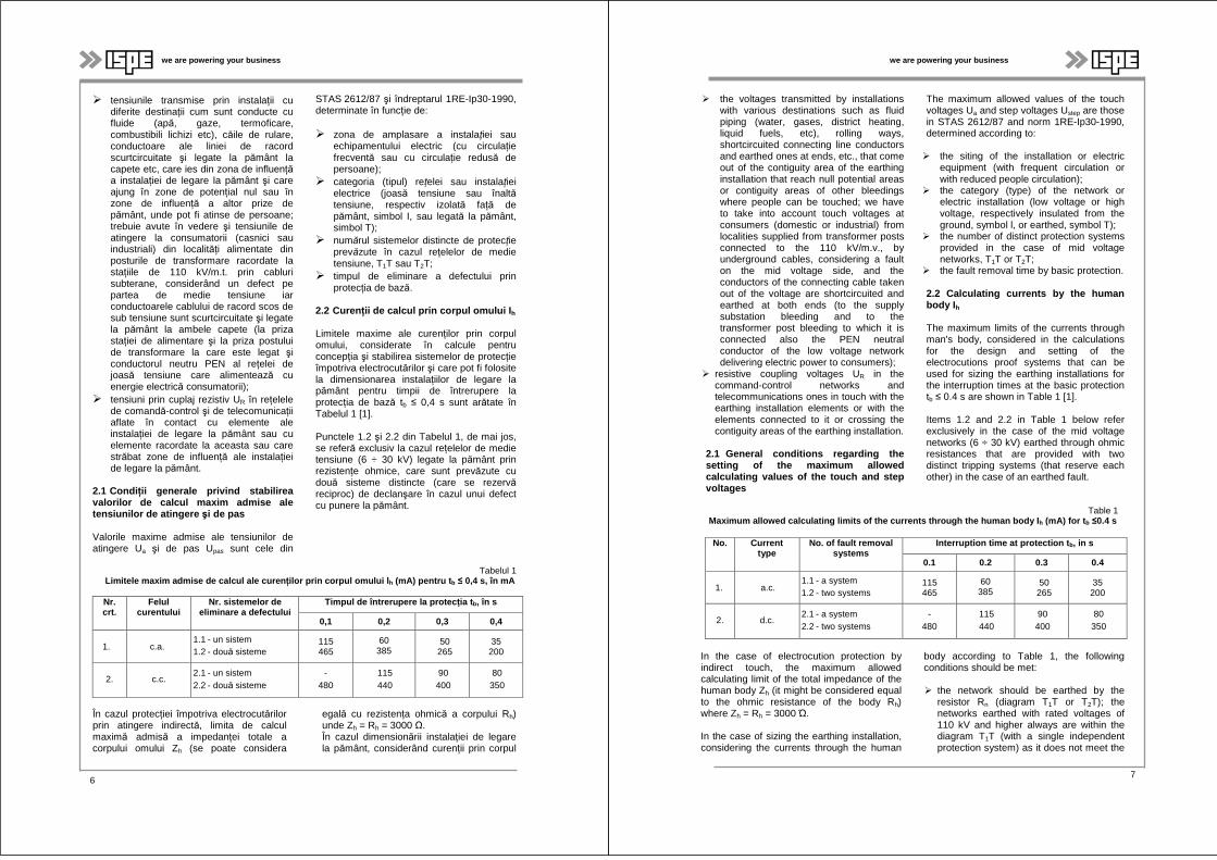
2.2 Curen ţii de calcul prin corpul omului I h
Limitele maxime ale curenţilor prin corpul omului, considerate în calcule pentru concepţia şi stabilirea sistemelor de protecţie împotriva electrocutărilor şi care pot fi folosite la dimensionarea instalaţiilor de legare la pământ pentru timpii de întrerupere la protecţia de bază tb ≤ 0,4 s sunt arătate în Tabelul 1 [1].
Punctele 1.2 şi 2.2 din Tabelul 1, de mai jos, se referă exclusiv la cazul reţelelor de medie tensiune (6 ÷ 30 kV) legate la pământ prin rezistenţe ohmice, care sunt prevăzute cu două sisteme distincte (care se rezervăreciproc) de declanşare în cazul unui defect cu punere la pământ.
Tabelul 1 Limitele maxim admise de calcul ale curen ţilor prin corpul omului l h (mA) pentru t b ≤ 0,4 s, în mA
Nr.crt.
Felul curentului
Nr. sistemelor de eliminare a defectului
Timpul de întrerupere la protec ţia tb, în s
0,1 0,2 0,3 0,4
1. c.a. 1.1 - un sistem 1.2 - două sisteme
115 465
60 385
50 265
35 200
2. c.c. 2.1 - un sistem 2.2 - două sisteme
- 480
115 440
90 400
80 350
În cazul protecţiei împotriva electrocutărilor prin atingere indirectă, limita de calcul maximă admisă a impedanţei totale a corpului omului Zh (se poate considera
egală cu rezistenţa ohmică a corpului Rh) unde Zh = Rh = 3000 Ω. În cazul dimensionării instalaţiei de legare la pământ, considerând curenţii prin corpul
6
we are powering your business
the voltages transmitted by installations with various destinations such as fluid piping (water, gases, district heating, liquid fuels, etc), rolling ways, shortcircuited connecting line conductors and earthed ones at ends, etc., that come out of the contiguity area of the earthing installation that reach null potential areas or contiguity areas of other bleedings where people can be touched; we have to take into account touch voltages at consumers (domestic or industrial) from localities supplied from transformer posts connected to the 110 kV/m.v., by underground cables, considering a fault on the mid voltage side, and the conductors of the connecting cable taken out of the voltage are shortcircuited and earthed at both ends (to the supply substation bleeding and to the transformer post bleeding to which it is connected also the PEN neutral conductor of the low voltage network delivering electric power to consumers);
resistive coupling voltages UR in the command-control networks and telecommunications ones in touch with the earthing installation elements or with the elements connected to it or crossing the contiguity areas of the earthing installation.
2.1 General conditions regarding the setting of the maximum allowed calculating values of the touch and step voltages
The maximum allowed values of the touch voltages Ua and step voltages Ustep are those in STAS 2612/87 and norm 1RE-Ip30-1990, determined according to:
the siting of the installation or electric equipment (with frequent circulation or with reduced people circulation);
the category (type) of the network or electric installation (low voltage or high voltage, respectively insulated from the ground, symbol l, or earthed, symbol T);
the number of distinct protection systems provided in the case of mid voltage networks, T1T or T2T;
the fault removal time by basic protection.
2.2 Calculating currents by the human body I h
The maximum limits of the currents through man's body, considered in the calculations for the design and setting of the electrocutions proof systems that can be used for sizing the earthing installations for the interruption times at the basic protection tb ≤ 0.4 s are shown in Table 1 [1].
Items 1.2 and 2.2 in Table 1 below refer exclusively in the case of the mid voltage networks (6 ÷ 30 kV) earthed through ohmic resistances that are provided with two distinct tripping systems (that reserve each other) in the case of an earthed fault.
Table 1 Maximum allowed calculating limits of the currents through the human body I h (mA) for t b ≤0.4 s
No. Current type
No. of fault removal systems
Interruption time at protection t b, in s
0.1 0.2 0.3 0.4
1. a.c. 1.1 - a system 1.2 - two systems
115 465
60 385
50 265
35 200
2. d.c. 2.1 - a system 2.2 - two systems
- 480
115 440
90 400
80 350
In the case of electrocution protection by indirect touch, the maximum allowed calculating limit of the total impedance of the human body Zh (it might be considered equal to the ohmic resistance of the body Rh) where Zh = Rh = 3000 Ώ.
In the case of sizing the earthing installation, considering the currents through the human
body according to Table 1, the following conditions should be met:
the network should be earthed by the resistor Rn (diagram T1T or T2T); the networks earthed with rated voltages of 110 kV and higher always are within the diagram T1T (with a single independent protection system) as it does not meet the
7
we are powering your business
omului conform Tabelului 1, trebuie să fie îndeplinite următoarele condiţii:
reţeaua să fie legată la pământ prin rezistor Rn (schema T1T sau T2T); reţelele legate la pământ cu tensiuni nominale de 110 kV şi mai mari se încadrează totdeauna în schema T1T (cu un singur sistem independent de protecţie) deoarece nu se îndeplineşte condiţionarea prevederii a douăsisteme de protecţie independente care să se rezerve reciproc;
tensiunea la care este supus omul, Uh
de calcul, trebuie să fie cel mult egalăcu valoarea maximă admisă a tensiunii de atingere Ua şi de pas Upas, stabilităde legislaţia în vigoare pentru situaţia respectivă (a se vedea 1):
Uh = Rh • Ih ≤ Ua şi
Rh • Ih ≤ Upas (1)
În cazul reţelelor cu două sisteme independente de eliminare a unui defect, curenţii maximi admişi prin corpul omului sunt mult mai mari decât în cazul reţelelor cu un singur sistem de eliminare a defectului. De exemplu, la un timp de întrerupere de 0,2 s valoarea uzuală la protecţiile homopolare de curent, curentul maxim admis la o reţea cu două sisteme independente de eliminare a defectului este lh = 385 mA, pe când la reţelele cu un singur sistem de eliminarea a defectului este Ih = 60 mA. De aici reies avantajele deosebite ale reţelelor din prima categorie menţionată mai sus. În primul rând,
condiţiile de dimensionare a prizelor de pământ vor fi mult mai uşoare, conducând la instalaţii mai simple, cu investiţii şi volume de lucru şi de materiale mult mai reduse.
2.3 Tensiuni de atingere U a şi de pas U pas
Valorile maxime admise pentru tensiunile de atingere şi de pas sunt cele indicate:
din Tabelul 2 pentru echipamentele (instalaţiile) electrice de înaltă tensiune (inclusiv medie tensiune) în cazul unui defect în instalaţia de înaltă tensiune în funcţie de tipul echipamentului (instalaţiei electrice), de zona de amplasare, de tipul reţelei şi de timpul de întrerupere în caz de defect;
în cazul folosirii în comun a instalaţiilor de protecţie (ca, de exemplu, cea de legare la pământ) pentru instalaţii sau echipamente electrice de înaltă şi joasătensiune: tensiunile de atingere şi de pas maxime admise pentru ambele categorii, sunt conform prevederilor din normativul I7-2011, când se considerădefectul pe partea de joasă tensiune şi cele din Tabelul 2, când se considerădefectul pe partea de înaltă tensiune.
În consecinţă dimensionarea instalaţiilor de legare la pământ pentru instalaţiile de ÎT se va realiza având la bază valorile normate ale tensiunilor maxim admise de atingere şi de pas, din Tabelul 2.
8
we are powering your business
conditioning of the provision regarding two independent protection systems that are in reciprocal standby;
the voltage to which man is subjected, calculating Uh, has to be at the most equal to the maximum allowed value of the touch Ua and step Ustep voltage, established by the curent legislation for the respective situation (see 1):
Uh = Rh • Ih ≤ Ua
and Rh • Ih ≤ Ustep (1)
In the case of the networks with two independent fault removal systems, the maximum allowed currents through the human body are much higher than in the case of the networks with a single fault removal system. For example, for an interruption time of 0.2 s the usual value at homopolar current protections, the maximum allowed current at a network with two independent fault removal systems is Ih = 385 mA, while for networks with a single fault removal system is In = 60 mA. Hence the special advantages of the networks of the first category mentioned above. Firstly, the sizing conditions of the bleedings will be much easier, leading to simpler installations, with investments and working and material volumes much reduced.................................
2.3 Touch U a and step U step voltages
The maximum allowed values for the touch and step voltages are those indicated:
in Table 2 for the high voltage power equipment (installations) in the case of a fault in the high voltage installation according to the type of equipment (power equipment), to the siting, the type of the network and the interruption time in case of fault;
in case of using jointly the protection installations (as, for example, the earthing one) for installations or high and low voltage power equipment the maximum allowed touch and step voltages for both categories, comply with the provisions in standard 17-2011, when it is considered that the fault on the low voltage side and those in Table 2, when it is considered the fault on the high voltage side.
Consequently, the sizing of the earthing installations for the HV installations will be carried out starting from the rated values of the maximum allowed touch and step voltages in Table 2.
9
we are powering your business
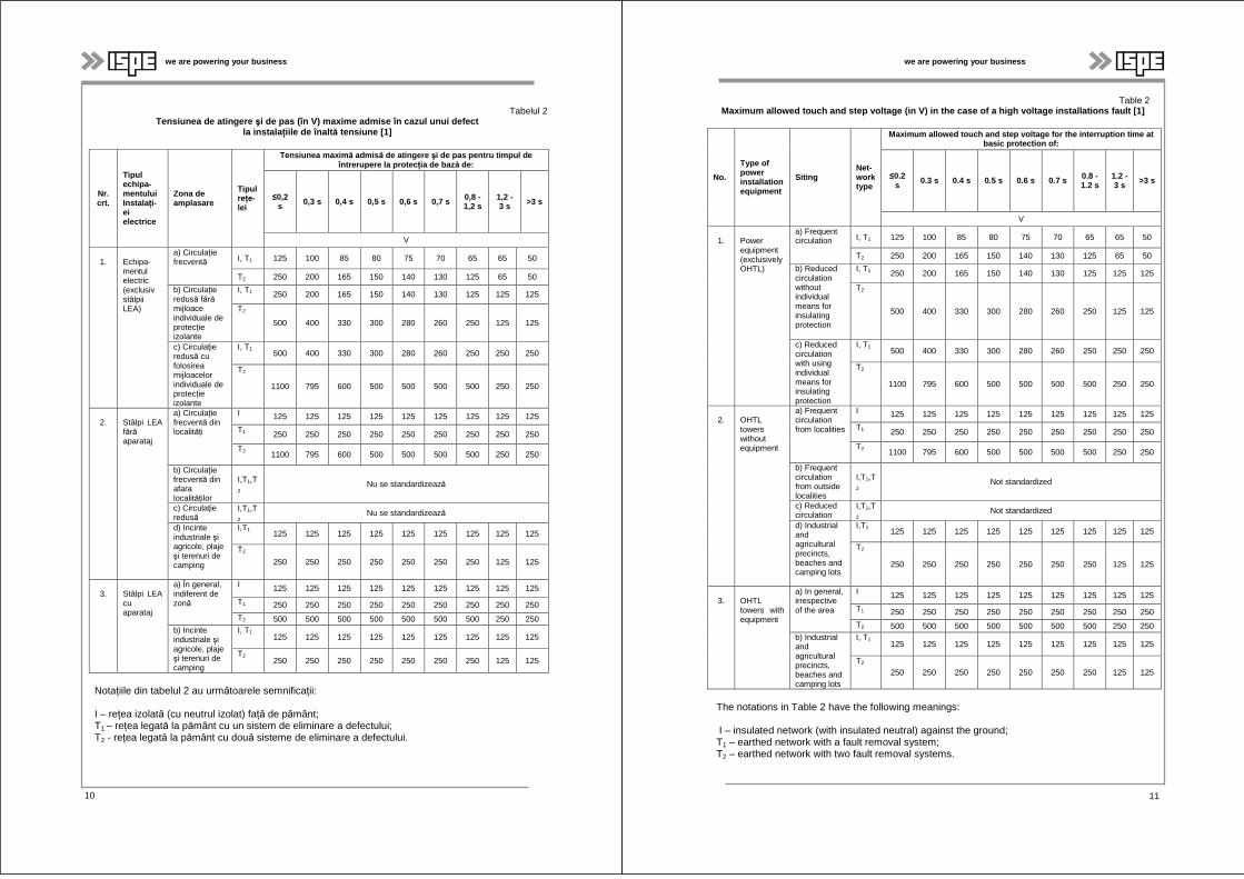
Tabelul 2 Tensiunea de atingere şi de pas (în V) maxime admise în cazul unui defect
la instala ţiile de înalt ă tensiune [1]
Nr. crt.
Tipul echipa-mentului Instala ţi-ei electrice
Zona de amplasare
Tipul reţe-lei
Tensiunea maxim ă admis ă de atingere şi de pas pentru timpul de întrerupere la protec ţia de baz ă de:
≤0,2 s 0,3 s 0,4 s 0,5 s 0,6 s 0,7 s 0,8 -
1,2 s 1,2 - 3 s >3 s
V
1. Echipa-mentul electric (exclusiv stâlpii LEA)
a) Circulaţie frecventă I, T1 125 100 85 80 75 70 65 65 50
T2 250 200 165 150 140 130 125 65 50
b) Circulaţie redusă fărămijloace individuale de protecţie izolante
I, T1 250 200 165 150 140 130 125 125 125
T2
500 400 330 300 280 260 250 125 125
c) Circulaţie redusă cu folosirea mijloacelor individuale de protecţie izolante
I, T1500 400 330 300 280 260 250 250 250
T2
1100 795 600 500 500 500 500 250 250
2. Stâlpi LEA fărăaparataj
a) Circulaţie frecventă din localităţi
I 125 125 125 125 125 125 125 125 125
T1 250 250 250 250 250 250 250 250 250
T2 1100 795 600 500 500 500 500 250 250
b) Circulaţie frecventă din afara localităţilor
I,T1,T2
Nu se standardizează
c) Circulaţie redusă
I,T1,T2
Nu se standardizează
d) Incinte industriale şi agricole, plaje şi terenuri de camping
I,T1125 125 125 125 125 125 125 125 125
T2
250 250 250 250 250 250 250 125 125
3. Stâlpi LEA cu aparataj
a) În general, indiferent de zonă
I 125 125 125 125 125 125 125 125 125
T1 250 250 250 250 250 250 250 250 250
T2 500 500 500 500 500 500 500 250 250 b) Incinte industriale şi agricole, plaje şi terenuri de camping
I, T1125 125 125 125 125 125 125 125 125
T2250 250 250 250 250 250 250 125 125
Notaţiile din tabelul 2 au următoarele semnificaţii:
I – reţea izolată (cu neutrul izolat) faţă de pământ; T1 – reţea legată la pământ cu un sistem de eliminare a defectului; T2 - reţea legată la pământ cu două sisteme de eliminare a defectului.
10
we are powering your business
Table 2 Maximum allowed touch and step voltage (in V) in the case of a high voltage installations fault [1]
No.
Type of power installation equipment
Siting Net- work type
Maximum allowed touch and step voltage for the inte rruption time at basic protection of:
≤0.2 s 0.3 s 0.4 s 0.5 s 0.6 s 0.7 s 0.8 -
1.2 s 1.2 - 3 s >3 s
V
1. Power equipment (exclusively OHTL)
a) Frequent circulation I, T1 125 100 85 80 75 70 65 65 50
T2 250 200 165 150 140 130 125 65 50
b) Reduced circulation without individual means for insulating protection
I, T1 250 200 165 150 140 130 125 125 125
T2
500 400 330 300 280 260 250 125 125
c) Reduced circulation with using individual means for insulating protection
I, T1 500 400 330 300 280 260 250 250 250
T2
1100 795 600 500 500 500 500 250 250
2. OHTL towers without equipment
a) Frequent circulation from localities
I 125 125 125 125 125 125 125 125 125
T1 250 250 250 250 250 250 250 250 250
T2 1100 795 600 500 500 500 500 250 250
b) Frequent circulation from outside localities
I,T1,T2
Not standardized
c) Reduced circulation
I,T1,T2
Not standardized
d) Industrial and agricultural precincts, beaches and camping lots
I,T1 125 125 125 125 125 125 125 125 125
T2
250 250 250 250 250 250 250 125 125
3. OHTL towers with equipment
a) In general, irrespective of the area
I 125 125 125 125 125 125 125 125 125
T1 250 250 250 250 250 250 250 250 250
T2 500 500 500 500 500 500 500 250 250 b) Industrial and agricultural precincts, beaches and camping lots
I, T1 125 125 125 125 125 125 125 125 125
T2
250 250 250 250 250 250 250 125 125
The notations in Table 2 have the following meanings:
I – insulated network (with insulated neutral) against the ground; T1 – earthed network with a fault removal system; T2 – earthed network with two fault removal systems.
11
we are powering your business
3. Dimensionarea instala ţiilor de legare la pământ, de ÎT, în conformitate cu standardul IEEE – ST 80
Efectele trecerii curentului electric prin părţile vitale ale corpului omului depind de durata, valoarea şi de frecvenţa curentului. Cea mai periculoasă consecinţă a unei asemenea expuneri este fibrilaţia ventriculară având ca rezultat oprirea circulaţiei sângelui. Dimensionarea instalaţiilor de legare la pământ este considerată nejustificată pentru preîntâmpinarea şocurilor puţin dureroase şi care nu cauzează leziuni serioase, acesta fiind cazul curenţilor mai mici decât pragul de fibrilaţie ventriculară (valoarea minimă a curentului prin corp care provoacă fibrilaţie ventriculară), astfel dimensionarea/proiecta-rea se realizează pornind de la valorile curenţilor maxim admişi care nu determinăfibrilaţii ventriculare.
3.1 Curen ţii admisibili prin corpul omului
Valoarea şi durata curenţilor care traversează corpul uman la frecvenţele de 50 Hz, respectiv 60 Hz trebuie să fie mai mici decât aceia care determină fibrilaţia ventriculară. Durata pentru care un curent, la frecvenţa de 50 Hz, respectiv 60 Hz, poate fi tolerat de majoritatea populaţiei este dată în principal de ecuaţia (2). Pe baza rezultatelor din studiul realizat de Dalziel, se presupune că99,5% din toată populaţia poate rezista, fărăriscul apariţiei fibrilaţiei ventriculare, la trecerea unui curent de mărimea şi durata prezentată în următoarea formulă de calcul:
s
Bt
kI = (2)
unde: k=k50 = 0,116 (pentru o persoană având aproximativ 50 kg). k=k70 = 0,157 (pentru o persoană având aproximativ 70 kg).
Relaţia (2) este bazată pe teste limitate la o valoare cuprinsă între 0,03÷3,0 secunde.
3.2 Rezisten ţa electric ă a corpului omului
Atât în curent continuu, cât şi în curent alternativ pentru frecvenţe normale (50÷60Hz) corpul omului poate fi reprezentat prin rezistenţe neinductive. Rezistenţa fiind măsurată între extremităţi: de la mână la
ambele picioare sau de la un picior la celălalt picior.
Astfel, se consideră următoarele:
rezistenţa pentru contactul mâinii şi al pantofului se consideră neglijabilă (egalăcu zero);
valoarea rezistenţei de 1000 Ω este aleasă pentru calcul şi este consideratăca fiind rezistenţa corpului uman de la mână la amândouă picioarele, de la mână la mână şi de la un picior la alt picior.
3.3 Circuitul echivalent în cazul unui defect
Rezistenţa circuitului de defect RA este funcţie de rezistenţa corpului uman RB şi de rezistenţa de pas Rpas (rezistenţa pământului de sub picior). Rezistenţa Rpas poate afecta apreciabil valoarea RA, fapt ce poate fi folositor în anumite cazuri. Pentru cazul circuitului analizat, tălpile picioarelor sunt în general reprezentate ca nişte discuri metalice conductoare iar contactul pantofului şi al şosetelor este neglijabil. Rezistenţa mutuală pentru două discuri metalice de raza b, poziţionate la o distanţădPas pe o suprafaţă de pământ considerat omogen, cu rezistivitatea ρ, este:
Rpas = ρ/(4·b) (3)
RMpas = ρ/(2·π·dPas) (4)
în care: Rpas – rezistenţa de dispersie proprie a fiecărui picior în contact cu pământul; RMpas – rezistenţa mutuală dintre cele douăpicioare; b – raza echivalentă a piciorului, în metri; dPas – distanţa dintre cele două picioare; ρ – rezistivitatea solului în contact cu picioarele omului. Rezistenţa de dispersie prin pământul în contact cu cele două picioare, în serie şi în paralel se poate scrie:
R2Ps= 2· (Rpas - RMpas) (5)
R2Pp= ½ · (R pas + RMpas) (6)
12
we are powering your business
3. Sizing the high voltage earthing installations according to the standard IEEE – ST 80
The effects of the electric current steping through the vital parts of the human body depend on the duration, value and frequency of the current. The most dangerous consequence of such an exposure is the ventricular fibrilation resulting in stopping blood circulation. The sizing of the earthing installations is considered unjustified for preventing less painful shocks that do not cause serious lesions, as the case with lower currents than the ventricular fibrilation threshold (minimum value of the current through the body provoking ventricular fibrilation), thus the sizing/designing is performed starting from the maximum allowed current values that do not determine ventricular fibrilation.
3.1 Allowed currents through the human body
The value and duration of the currents crossing the human body at frequencies of 50 Hz, 60 Hz, respectively, have to be lower than those determining ventricular fibrilation. The duration for which a current, at the frequency of 50 Hz, 60 Hz, respectively, can be tolerated by most people is given mainly by the equation (2). Based on the results from the study conducted by Dalziel, it is presupposed that 99.5% of the whole population can resist without the risk of ventricular fibrilation occurring, at the steping of a current of the size and duration presented in the following calculating formula:
s
Bt
kI = (2)
where: k=k50 = 0.116 (for a person weighing about 50 kg). k=k70 = 0.157 (for a person weighing about 70 kg).
The relation (2) is based on the tests limited to a value ranging between 0.03÷3.0 seconds.
3.2 Electrical resistance of the human body
Both in direct current and in alternative current for the regular frequencies (50÷60Hz) the human body can be represented by noninductive resistances. As the resistance is measured between ends from the hands to both feet or from a foot to the other foot. Thus the following are considered:
the resistance for the touch of the hand and of the shoe is considered to be negligible (equal to zero);
the resistance value of 1000 Ω is chosen for calculation and is considered as the resistance of the human body from the hand to both feet, from hand to hand and from a foot to another foot.
3.3 The equivalent circuit in case of a fault
The resistance of a fault circuit RA depends on the resistance of the human body RB and the step resistance Rstep (the resistance of the ground under the foot). The resistance Rstep can affect considerably the value RA, which can be useful in certain cases. For the case of the analyzed circuit, the soles of the feet usually are represented like conducting metallic discs, and the touch of the shoe and socks is negligible. The mutual resistance for two metallic discs of ray b, located at a distance dstep on a ground surface considered to be homogeneous, with resistivity ρ, is:
Rstep = ρ/(4·b) (3)
RMstep = ρ/(2·π·dstep) (4)
where: Rstep – the own dispersion resistance of each foot in touch with the ground; Rmstep – the mutual resistance between the two feet; b – the equivalent ray of the foot, in meters; dstep – the distance between the two feet; ρ – the ground resistivity in touch with the human feet. The dispersion resistance through the earth in touch with the two feet, in series and in parallel can be written:
R2Ps= 2· (Rstep - RMstep) (5)
R2Pp= ½ · (R step + RMstep) (6)
13
we are powering your business
unde: R2Ps – rezistenţa pentru cazul în care cele două picioare sunt în serie (cazul tensiunii de pas); R2Pp – rezistenţa pentru cazul în care cele două sunt în paralel (cazul tensiunii de atingere între o mână şi picioarele omului).
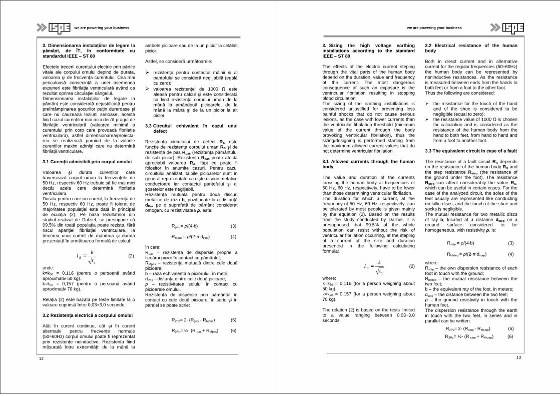
În Figura 1 este arătat circuitul echivalent pentru contactul picior – picior. Tensiunea de pas Upas, aplicată corpului uman, reprezintădiferenţa de potenţial maximă admisă dintre două puncte accesibile de pe suprafaţa solului, aflate la o distanţă de un pas (se consideră 1 m),
unde: dPas = 1 m; RA = RB + 2 · RPas -2 · RMpas; - rezistenţa echivalentă pentru circuitul considerat. IA = U/RA; - curentul prin circuitul accidental. RB= 1000 Ω.
Rezistenţa echivalentă pentru circuitul tensiunii de pas se mai poate scrie şi ca:
RA = RB + 2 · (Rpas - RMpas) (7) Circuitul echivalent pentru tensiunea de atingere este arătat în figura 2.
Fig. 2 - Circuitul echivalent aferent tensiunii de atingere [3]
Astfel având în vedere circuitul echivalent de mai sus (Figura 2), rezistenţa echivalentăpentru circuitul tensiunii de atingere se poate scrie şi ca:
RA = RB + 1/2 · (Rpas + RMpas) (8)
Cărţile de specialitate consideră raza echivalentă a discului care echivalează pasul omului de 0,08 m şi neglijează rezistenţa mutuală. Având în vedere aceste simplificări se pot rescrie ecuaţiile (5) şi (6), funcţie de
rezistivitatea solului, şi anume rezistenţa de dispersie prin pământul în contact cu cele două picioare, în serie şi în paralel:
R2Ps= 6·ρ (9)
R2Pp= 1,5 · ρ (10)
Ţinând seama de cele prezentate în capitolul 3 se pot scrie următoarele relaţii general valabile pentru determinarea tensiunilor maxim admise de atingere şi de pas (a se vedea tabelul 3) în care:
Fig. 1 – Circuitul echivalent aferent tensiuni de p as [3]
14 14
we are powering your business
where: R2Ps – the resistance for the case in which the two feet are in series (the case of the step voltage); R2Pp – the resistance for the case in which the two are in parallel (the case of the touch voltage between a hand and the human feet).
In Figure 1 we show the equivalent circuit for the foot – foot touch. The step voltage Ustep, applied to the human body, represents the maximum allowed potential diference between the two points accessible from the surface of the ground, found at a distance of a step (it is considered 1 m).
Fig. 1 - Equivalent circuit corresponding to the st ep voltage [3]
where: dStep = 1 m; RA = RB + 2 · RStep -2 · RMstep; - equivalent resistance for the considered circuit. IA = U/RA; - the current through the accidental circuit. RB= 1000 Ω.
The equivalent resistance for the step voltage circuit can be written also like:
RA = RB + 2 · (Rstep - RMstep) (7)
The equivalent resistance for the touch voltage is shown in Figure 2.
Fig. 2 - The equivalent circuit of the touch volta ge [3]
Thus, taking into account the equivalent circuit above (Figure 2), the equivalent resistance for the touch voltage circuit can be written also like:
RA = RB + 1/2 · (Rstep + RMstep) (8)
The speciality books consider the equivalent ray of the disc equalling man's step of 0.08 m and neglects mutual resistance. Taking into account these simplifications we can rewrite the equations (5) and (6), depending on the resistivity of the ground,
namely the dispersion resistance through the earth in touch with the two feet, in series and in parallel:
R2Ps= 6·ρ (9)
R2Pp= 1,5 · ρ (10)
Taking into account those presented in chapter 3 we can write the following generally valid relations for determining the maximum allowed touch and step voltages (see Table 3) in which:
15
we are powering your business
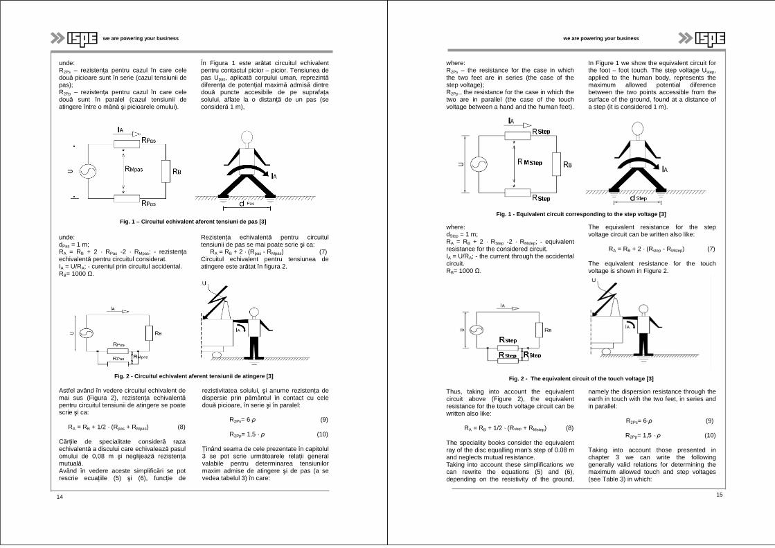
Tabelul 3 [3]
Tensiunea de atingere maxim ăadmis ă
Tensiunea de pas maxim ă admis ă
Masa corpului 5 0 kg (folosit pentru zone publice – circula ţie frecvent ă)
s
ssa
t
CU
ρ⋅⋅+=
174,0116
s
sspas
t
CU
ρ⋅⋅+=
696,0116
Masa corpului 70 kg (folosit pentru zone restric ţionate - cu circula ţie redus ă)
s
ssa
t
CU
ρ⋅⋅+=
236,0157
s
sspas
t
CU
ρ⋅⋅+=
942,0157
unde:
Cs = 1 pentru cazul în care nu există nici un strat de piatră spartă sau este determinat din diagramele din ST80 dacă există un strat de piatră spartă cu rezistivitate ridicată; ρs = rezistivitatea solului în Ω · m; ts = durata şocului de curent în secunde. Astfel pentru a realiza o comparaţie între valorile tensiunilor de atingere şi de pas maxim admise propuse de IEEE cu valorile tensiunilor maxim admise de atingere şi de pas indicate în standardele româneşti şi descrise în capitolul 2, se vor calcula valorile
tensiunilor folosind formulele din tabelul 3, luând în considerare următoarele ipoteze: - rezistenţa electrică a corpului omului este considerată 1000 Ω; - nu se consideră izolarea amplasamentului (Cs = 1); - rezistivitatea echivalentă a solului este considerată 100 Ωm;
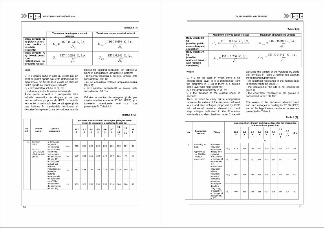
Valorile tensiunilor de atingere şi de pas maxim admise conform ST 80 (IEEE) şi a ipotezelor menţionate mai sus sunt prezentate în Tabelul 4.
Tabelul 4 [5]
Nr. crt.
Metodăcalcul
Zonă de amplasare
Tensiunea maxim ă admis ă de atingere şi de pas pentru timpul de întrerupere la protec ţia de baz ă de:
≤0,2 s
0,3 s
0,4 s
0,5 s
0,6 s
0,7 s
0,8 -
1,2 s
1,2 -
3 s
>3 s
V
1. Conform IEEE
Ipoteze: - ρ= 100 Ωm; - fără strat de pietriş;
a) Circulaţie frecventă(corespunză-tor pentru un corp 50 kg) Independent de tipul reţelei (IT sau TT)
Upas 415 338 293 262 239 221 169 107 83
Ua 298 243 210 188 172 159 121 77 59
b) Circulaţie redusă fărămijloace individuale de protecţie izolante (corespunză-tor pentru un corp 70 kg) Independent de tipul reţelei (IT sau TT)
Upas 561 458 397 355 324 300 229 145 112
Ua 403 329 285 255 233 215 164 104 80
16
we are powering your business
Table 3 [3]
Maximum allowed touch voltage Maximum allowed step voltageBody weight 50 kg (used for public areas – frequent circulation)
s
ssa
t
CU
ρ⋅⋅+=
174.0116
s
ssstep
t
CU
ρ⋅⋅+=
696.0116
Body weight 70 kg (used for restricted areas –with reduced circulation)
s
ssa
t
CU
ρ⋅⋅+= 236.0157s
ssstep
t
CU
ρ⋅⋅+=
942.0157
where:
Cs = 1 for the case in which there is no broken stone layer or it is determined from the diagrams in ST80 if there is a broken stone layer with high resistivity; ρs = the ground resistivity in Ω · m; ts = the duration of the current shock in seconds. Thus, in order to carry out a comparison between the values of the maximum allowed touch and step voltages proposed by IEEE with values of maximum allowed touch and step voltages indicated in the Romanian standards and described in chapter 2, we will
calculate the values of the voltages by using the formulas in Table 3, taking into account the following hypotheses: - the electrical resistance of the human body is considered to be 1000 Ω; - the insulation of the site is not considered (Cs = 1). - the equivalent resistivity of the ground is considered to be 100 Ωm.
The values of the maximum allowed touch and step voltages according to ST 80 (IEEE) and of the hypotheses mentioned above are presented in Table 4.
Table 4 [5]
No. Calculation method Siting
Maximum allowed touch and step voltages for the int erruption time at the basic protection:
≤0.2 s
0.3 s
0.4 s
0.5 s
0.6 s
0.7 s
0.8 -
1.2 s
1.2 -
3 s >3 s
V
1. According to IEEE
Hypotheses: - ρ= 100 Ωm; - without gravel layer;
a) Frequent circulation (correspon-ding to a 50 kg body) Irrespective of the type of network (HV or TT)
Ustep 415 338 293 262 239 221 169 107 83
Ua 298 243 210 188 172 159 121 77 59
b) Reduced circulation without individual means of insulating protection (correspon-ding to a 70kg body) Irrespective of the type of network (HV or TT)
Ustep 561 458 397 355 324 300 229 145 112
Ua 403 329 285 255 233 215 164 104 80
17
we are powering your business
4. Rezisten ţa instala ţiilor de legare la pământ
Având în vedere relaţiile din tabelul 3 rezistenţa instalaţiei de legare la pământ aferentă incintelor restricţionate (cu circulaţie redusă) trebuie să fie mai mică sau egală cu:
Rpriza ≤priza
a
I
U (11)
Rpriza ≤priza
pas
I
U (12)
5. Concluzii
Asigurarea siguranţei personalului de exploatare precum şi a funcţionării instalaţiilor electrice depind în mare măsurăde o dimensionare corespunzătoare a instalaţiilor de legare la pământ care le deservesc. Conform practicii din România valorile tensiunile de atingere şi de pas sunt standardizate, şi egale, şi se aplică indiferent de tipul solului (rezistivitatea solului), pe când în standardul american IEEE, acestea sunt diferenţiate (tensiunea de atingere diferită de tensiunea de pas), lăsând la îndemâna proiectantului să determine valorile tensiunilor de atingere şi de pas în funcţie de
amplasamentul (tipul solului – rezistivitatea acestuia) instalaţiei electrice. Totodatăstandardul american (ST80 – IEEE) nu ţine cont de tipul reţelei (I, T1, T2). Din compararea valorilor tensiunilor maxim admise de atingere şi de pas din cele douătabele 2 şi 4, în ipotezele menţionate, se observă că pentru valori ale timpului de întrerupere al protecţiei de bază mai mici decât 0,8 s şi pentru reţele de tip I, T1
(conform practicii româneşti) valorile tensiunilor de atingere şi de pas calculate conform IEEE sunt mai mari conducând la o dimensionare a instalaţilor de legare la pământ mai economică fără a pune în pericol viaţa omului.
În urma acestui studiu comparativ reiese necesitatea revizuirii legislaţiei româneşti specifice dimensionării instalaţiilor de legare la pământ (STAS 2612, 1 RE Ip 30), în special a valorilor tensiunilor de atingere şi de pas maxim admise, valori care au fost calculate, având la bază ipoteze care pentru momenul de faţă sunt perimate (curenţi maxim admisibili prin corpul omului, rezistenţa corpului omului pentru diferite trasee ale curentului). Modificarea acestor valori ale tensiunilor de atingere şi de pas maxim admise va conduce la o dimensionarea optimă din punct de vedere tehnico-economic.
Bibliografie
[1] 1RE Ip 30 – 1990 Îndreptar de proiectare şi execuţie a instalaţiilor de legare la pământ; [2] Mauriciu Sufrim, Miron Laurenţiu Goia, Mircea Petran, Instalaţii de legare la pământ. Editura Tehnică, Bucureşti 1987; [3] *** IEEE Std. 80-2000 şi 1986, IEEE Guide for safety in AC substation groundig; [4] *** IEC/TS 60479-1_ed 4/2005-07, Partea 1: Aspecte generale, Efectele curentului electric asupra omului şi animalelor domestice; [5] Alexandru Dina, Teză de Doctorat – Contribuţii privind optimizarea tratării neutrului în reţelele de medie tensiune din România. Bucureşti 2011.
Referent: Consilier tehnico-economic ing. Maria Diaconescu
18
we are powering your business
4. Resistance of the earthing installations
Taking into account the relations in Table 3 the resistance of the earthing installation corresponding to the restricted precincts (with reduced circulation) should be lower or equal to:
Rsocket ≤socket
aI
U (11)
Rsocket ≤socket
step
I
U (12)
5. Conclusions
Ensuring the safety of the operating personnel as well as the operation of the power installations depends to a large extent on an adequate sizing of the earthing installations serving them. According to the Romanian practice the values of the touch and step voltages are standardized, and equal, and are applied irrespective of the type of ground (resistivity of the ground), while in the American standard IEEE, these are differentiated (the touch voltage differs from the step voltage), leaving at the disposal of the designer to determine the values of the touch and step voltages depending on the siting (type of
ground – its resistivity) of the power installation. At the same time, the American standard (ST80 – IEEE) does not take into account the type of network (I, T1, T2). From the comparison of the values of maximum allowed touch and step voltages in the two Tables 2 and 4, in the mentioned hypotheses, it is noticed that for the values of the interruption time of the basic protection lower than 0.8 s and for the networks of the I, T type (according to Romanian practice) the values of the touch and step voltages calculated according to IEEE are higher leading to a more economical sizing of the earthing installations without endangering human life.
In view of this comparative study it results that the review of the Romanian legislation specific of the sizing of earthing installations (STAS 2612, 1 RE Ip 30), especially the values of the maximum allowed touch and step voltages, values that were calculated, underlying hypotheses that for the time being are obsolete (maximum allowed currents through the human body, the resistance of the human body for various current paths). The change in these values of the maximum allowed touch and step voltages will lead to an optimum sizing from a technico-economic point of view.
References
[1] 1RE Ip 30 – 1990 Îndreptar de proiectare şi execuţie a instalaţiilor de legare la pământ; [2] Mauriciu Sufrim, Miron Laurenţiu Goia, Mircea Petran, Instalaţii de legare la pământ. Editura Tehnică, Bucureşti 1987 [3] *** IEEE Std. 80-2000 şi 1986, IEEE Guide for safety in AC substation groundig [4] *** IEC/TS 60479-1_ed 4/2005-07, Partea 1: Aspecte generale, Efectele curentului electric asupra omului şi animalelor domestice [5] Alexandru Dina, Teză de Doctorat – Contribuţii privind optimizarea tratării neutrului în reţelele de medie tensiune din România. Bucureşti 2011
Reviewer: Technico-economic counsellor eng. Maria Diaconescu
19
we are powering your business
EPURAREA APELOR UZATE ÎN BAZINE DE TIP MBBR
Ioana Corina MOGA 1
Irina VODĂ 2
Rezumat: În prezentul referat se prezintă un model matematic ce poate fi implementat în programe de calcul specializate, pentru determinarea concentraţiei de oxigen dizolvat din cadrul unor bioreactoare de tip Moving Bed Biofilm Reactor (MBBR), plecând de la ecuaţia generală a dispersiei. Scopul cercetărilor este de a determina poziția optimă a sistemului de aerare în interiorul bioreactorului, astfel încât concentrația de
oxigen dizolvat din masa de apă uzată să fie situată în limitele indicate de literatura de specialitate. De asemenea, se prezintă și rezultatele unor seturi de cercetări experimentale realizate pe un bazin de tip MBBR. Concentraţia de oxigen dizolvat este determinată experimental pentru un sistem de aerare cu ţevi perforate cu orificii de 2 mm.
Cuvinte cheie: epurare, oxigenare, elemente mobile, modelare matematic ă, simul ări numerice
1. Introducere
Analiza statistică a situaţiei principalelor surse de ape uzate în România, efectuatăpentru anul 2005, a relevat următoarele aspecte globale:
- Dintr-un volum total evacuat de 4.034,808 milioane m3/an, 65,1%, constituie ape uzate care trebuie epurate. - Din volumul total de ape uzate necesitând epurare şi anume, 2.626,139 milioane m3/an, circa 20,5%, a fost suficient (corespunzător) epurat. În rest, circa 45%, reprezintă ape uzate neepurate şi circa 34% ape uzate insuficient epurate. Prin urmare în anul 2005, cca. 79% din apele uzate, provenite de la principalele surse de poluare, au ajuns în receptorii naturali, în special râuri, neepurate sau insuficient epurate. - Referitor la aportul de ape uzate repartizat pe activităţi din economia naţională cel mai mare volum de ape uzate, inclusiv cele „convenţional curate“, a fost evacuat de unităţi din domeniile: Energie electrică şi termică: - peste 51%; Gospodărie comunală: peste 36%; Prelucrări chimice: - cca. 5%, Industrie metalurgică şi construcţii de maşini: - cca. 3%.
- Din punct de vedere al apelor uzate necesitând epurare, cele mai mari volume au fost evacuate în cadrul activităţilor: Gospodărie comunală: - peste 56%; Prelucrări chimice: - peste 7%; Industrie metalurgică şi construcţii de maşini: - peste 4%. - Cele mai mari volume de ape uzate neepurate, provin de la unităţi din domeniile: Gospodărie comunală: - cca. 49,05%. Cu o contribuţie mult mai redusă, se înscriu unităţile din cadrul activităţii Prelucrări chimice: - cca. 2%. - Referitor la apele uzate insuficient epurate, activităţile cu cea mai mare pondere se ordonează astfel: Gospodărie comunală: - cca. 62%; Prelucrări chimice: - cca. 11%; Industrie extractivă: - peste 2,6%; Industrie metalurgică şi construcţii de maşini: - cca. 2,4%; Industria de prelucrare a lemnului: - peste 2,3%. - Impactul surselor de poluare asupra receptorilor naturali depinde în afară de debitul efluent şi de încărcarea cu substanţe poluante.
Faţă de numărul total de 1.310 de staţii şi instalaţii de epurare şi stocare investigate în anul 2005, 492 de staţii, reprezentând 37,6%, au funcţionat corespunzător, iar restul de 818 staţii, adică 63,4%, necorespunzător.
1 Cercetător Ştiinţific III dr.ing., Universitatea Politehnica din Bucureşti 2 Cercetător Ştiinţific dr.ing., Secţia Studii Finanţare Proiecte, Institutul de Studii şi Proiectări Energetice – I.S.P.E. S.A.
20
we are powering your business
WASTE WATER TREATMENT IN THE MBBR BASINS
Ioana Corina MOGA 1 Irina VODĂ2
Summary: In the present paper we present a mathematical model that can be implemented in specialized computer programs, to determine the dissolved oxygen concentration within the MBBR (Moving Bed Biofilm Reactor) bioreactors, starting from the general equation of the dispersion. The goal of the researchers is to determine the optimum position of the airing system inside the bioreactor, so that the dissolved oxygen
concentration in the waste water mass be situated within the limits indicated in the specialized literature. At the same time, we present also the results of experimental researches sets carried out on a MBBR basin. The dissolved oxygen concentration is determined experimentally for an airing system with perforated piping with 2 mm orifices.
Key words: treatment, oxygenation, mobile elements, mathematical modelling, numerical simulations
1. Introduction
The statistical analysis of the situation of the main waste water sources in Romania, conducted in the year 2005, revealed the following global aspects:
- A total discharged volume of 4,034.808 million m3/year, 65.1%, constitute waste water that have to be treated.
- From the total waste water volume requiring treatment, that is, 2,626.139 million m3/year, about 20.5%, was sufficiently treated (adequately). For the rest, that is about 45%, are untreated waste waters and about 34%, insufficiently treated waste water. Consequently, in 2005, about 79% of the waste water, coming from the main polluting sources, reached the natural receivers, especially rivers, untreated or insufficiently treated.
- Regarding the waste water intake distributed by national economy activities the largest waste water volume, including those “conventionally clean”, was discharged by units in the fields: Electric and thermal power: - over 51%; Town administration: - over 36%; Chemical processing: - about 5%; Metallurgy industry and machine construction: about 3%.
- From the point of view of waste water requiring treatment, the largest volumes were discharged within the activities; Town administration: – over 56%; Chemical processing: - 7%; Metallurgy industry and machine construction: - over 4%.
- The largest untreated waste water volumes come from units in the fields: Town administration: – about 49.05%. A much reduced contribution have the units within the Chemical processing activities: - about 2%.
- Regarding the insufficiently treated waste water, the activities with the highest share are ordered as follows: Town administration: – about 62%; Chemical processing: – about 11%; Oil extractive industry: – over 2.6%; Metallurgy industry and machine construction: – about 2.4%; Wood processing industry: – over 2.3%.
- The impact of polluting sources upon natural receivers depends outside the effluent flowrate and the charging with polluting substances.
1SR III, Ph.D., Politehnica University in Bucharest 2 CS, Ph.D., Energy & Environment Division, Institute for Studies and Power Engineering – I.S.P.E. S.A.
21 21
we are powering your business
În acest context este necesar să se răspundăunor probleme grave cu care se confruntăRomânia şi anume, să se găsească metode adecvate de epurare a apelor uzate. Astfel se analizează utilizarea tehnologiei Mobile Bed Biofilm Reactor (MBBR) în cadrul proceselor de epurare biologică, ţinând seama ca aceasta este considerată în literatura de specialitate una dintre cele mai eficiente la nivel mondial.
2. Epurarea cu film biologic
Cele mai recente cercetări și tehnologii de epurare biologică se bazează pe fixarea
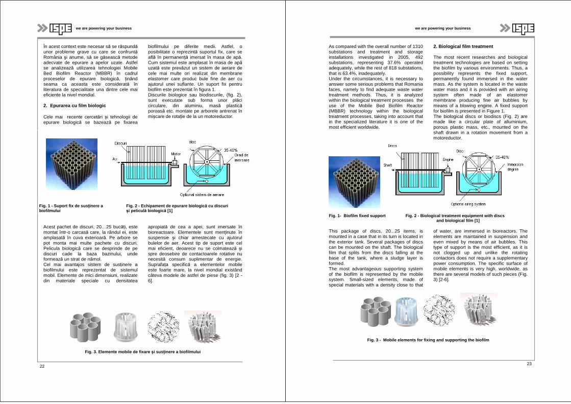
biofilmului pe diferite medii. Astfel, o posibilitate o reprezintă suportul fix, care se află în permanență imersat în masa de apă. Cum sistemul este amplasat în masa de apăuzată este prevăzut un sistem de aerare de cele mai multe ori realizat din membrane elastomer care produc bule fine de aer cu ajutorul unei suflante. Un suport fix pentru biofilm este prezentat în figura 1. Discurile biologice sau biodiscurile, (fig. 2), sunt executate sub forma unor plăci circulare, din aluminiu, masă plasticăporoasă etc. montate pe arborele antrenat în mișcare de rotație de la un motoreductor.
Fig. 1 - Suport fix de sus ținere a biofilmului
Fig. 2 - Echipament de epurare biologic ă cu discuri și pelicul ă biologic ă [1]
Acest pachet de discuri, 20…25 bucăți, este montat într-o carcasă care, la rândul ei, este amplasată în cuva exterioară. Pe arbore se pot monta mai multe pachete cu discuri. Pelicula biologică care se desprinde de pe discuri cade la baza bazinului, unde formează un strat de nămol. Cel mai avantajos sistem de susținere a biofilmului este reprezentat de sistemul mobil. Elemente de mici dimensiuni, realizate din materiale speciale cu densitatea
apropiată de cea a apei, sunt imersate în bioreactoare. Elementele sunt menținute în suspensie și chiar amestecate cu ajutorul bulelor de aer. Acest tip de suport este cel mai eficient, deoarece nu se colmatează și spre deosebire de contactoarele rotative nu necesită consum suplimentar de energie. Suprafața specifică a elementelor mobile este foarte mare, la nivel mondial existând câteva modele de astfel de piese (fig. 3) [2 - 6].
Fig. 3. Elemente mobile de fixare și sus ținere a biofilmului
22
we are powering your business
As compared with the overall number of 1310 substations and treatment and storage installations investigated in 2005, 492 substations, representing 37.6% operated adequately, while the rest of 818 substations, that is 63.4%, inadequately. Under the circumstances, it is necessary to answer some serious problems that Romania faces, namely to find adequate waste water treatment methods. Thus, it is analyzed within the biological treatment processes the use of the Mobile Bed Biofilm Reactor (MBBR) technology within the biological treatment processes, taking into account that in the specialized literature it is one of the most efficient worldwide.
2. Biological film treatment
The most recent researches and biological treatment technologies are based on setting the biofilm by various environments. Thus, a possibility represents the fixed support, permanently found immersed in the water mass. As the system is located in the waste water mass and it is provided with an airing system often made of an elastomer membrane producing fine air bubbles by means of a blowing engine. A fixed support for biofilm is presented in Figure 1. The biological discs or biodiscs (Fig. 2) are made like a circular plate of alluminium, porous plastic mass, etc., mounted on the shaft drawn in a rotation movement from a motoreductor.
Fig. 1- Biofilm fixed support Fig. 2 - Biological treatment equipment with discs and biolog ical film [1]
This package of discs, 20...25 items, is mounted in a case that in its turn is located in the exterior tank. Several packages of discs can be mounted on the shaft. The biological film that splits from the discs falling at the base of the tank, where a sludge layer is formed. The most advantageous supporting system of the biofilm is represented by the mobile system. Small-sized elements, made of special materials with a density close to that
of water, are immersed in bioreactors. The elements are maintained in suspension and even mixed by means of air bubbles. This type of support is the most efficient, as it is not clogged up and unlike the rotating contactors does not require a supplementary power consumption. The specific surface of mobile elements is very high, worldwide, as there are several models of such pieces (Fig. 3) [2-6].
Fig. 3 - Mobile elements for fixing and supporting the biofilm
23
we are powering your business
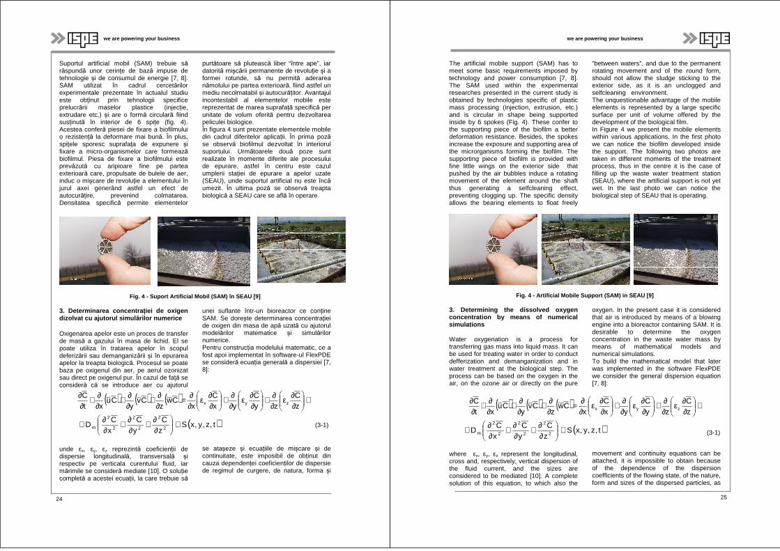
Suportul artificial mobil (SAM) trebuie sărăspundă unor cerințe de bază impuse de tehnologie și de consumul de energie [7, 8]. SAM utilizat în cadrul cercetărilor experimentale prezentate în actualul studiu este obținut prin tehnologii specifice prelucrării maselor plastice (injecție, extrudare etc.) și are o formă circulară fiind susținută în interior de 6 spiţe (fig. 4). Acestea conferă piesei de fixare a biofilmului o rezistență la deformare mai bună. În plus, spițele sporesc suprafața de expunere și fixare a micro-organismelor care formeazăbiofilmul. Piesa de fixare a biofilmului este prevăzută cu aripioare fine pe partea exterioară care, propulsate de bulele de aer, induc o mișcare de revoluție a elementului în jurul axei generând astfel un efect de autocurățire, prevenind colmatarea. Densitatea specifică permite elementelor
purtătoare să plutească liber “între ape”, iar datorită mișcării permanente de revoluție și a formei rotunde, să nu permită aderarea nămolului pe partea exterioară, fiind astfel un mediu necolmatabil și autocurățitor. Avantajul incontestabil al elementelor mobile este reprezentat de marea suprafață specifică per unitate de volum oferită pentru dezvoltarea peliculei biologice. În figura 4 sunt prezentate elementele mobile din cadrul diferitelor aplicații. În prima pozăse observă biofilmul dezvoltat în interiorul suportului. Următoarele două poze sunt realizate în momente diferite ale procesului de epurare, astfel în centru este cazul umplerii stației de epurare a apelor uzate (SEAU), unde suportul artificial nu este încăumezit. În ultima poză se observă treapta biologică a SEAU care se află în operare.
Fig. 4 - Suport Artificial Mobil (SAM) în SEAU [9]
3. Determinarea concentra ției de oxigen dizolvat cu ajutorul simul ărilor numerice
Oxigenarea apelor este un proces de transfer de masă a gazului în masa de lichid. El se poate utiliza în tratarea apelor în scopul deferizării sau demanganizării și în epurarea apelor la treapta biologică. Procesul se poate baza pe oxigenul din aer, pe aerul ozonizat sau direct pe oxigenul pur. În cazul de față se consideră că se introduce aer cu ajutorul
unei suflante într-un bioreactor ce conține SAM. Se dorește determinarea concentrației de oxigen din masa de apă uzată cu ajutorul modelărilor matematice și simulărilor numerice. Pentru construcția modelului matematic, ce a fost apoi implementat în software-ul FlexPDE se consideră ecuația generală a dispersiei [7, 8]:
( ) ( ) ( ) +
∂∂ε
∂∂+
∂∂ε
∂∂+
∂∂ε
∂∂=
∂∂+
∂∂+
∂∂+
∂∂
zC
zyC
yxC
xCw
zCv
yCu
xtC
zyx
( )t,z,y,xSzC
yC
xC
D 2
2
2
2
2
2
m +
∂∂+
∂∂+
∂∂+ (3-1)
unde εx, εy, εz reprezintă coeficienții de dispersie longitudinală, transversală și respectiv pe verticala curentului fluid, iar mărimile se consideră mediate [10]. O soluție completă a acestei ecuații, la care trebuie să
se atașeze și ecuațiile de mișcare și de continuitate, este imposibil de obținut din cauza dependenței coeficienților de dispersie de regimul de curgere, de natura, forma și
24
we are powering your business
The artificial mobile support (SAM) has to meet some basic requirements imposed by technology and power consumption [7, 8]. The SAM used within the experimental researches presented in the current study is obtained by technologies specific of plastic mass processing (injection, extrusion, etc.) and is circular in shape being supported inside by 6 spokes (Fig. 4). These confer to the supporting piece of the biofilm a better deformation resistance. Besides, the spokes increase the exposure and supporting area of the microrganisms forming the biofilm. The supporting piece of biofilm is provided with fine little wings on the exterior side that pushed by the air bubbles induce a rotating movement of the element around the shaft thus generating a selfcleaning effect, preventing clogging up. The specific density allows the bearing elements to float freely
“between waters”, and due to the permanent rotating movement and of the round form, should not allow the sludge sticking to the exterior side, as it is an unclogged and selfcleaning environment. Kkk kmkkkkkkkThe unquestionable advantage of the mobile elements is represented by a large specific surface per unit of volume offered by the development of the biological film. In Figure 4 we present the mobile elements within various applications. In the first photo we can notice the biofilm developed inside the support. The following two photos are taken in different moments of the treatment process, thus in the centre it is the case of filling up the waste water treatment station (SEAU), where the artificial support is not yet wet. In the last photo we can notice the biological step of SEAU that is operating.
Fig. 4 - Artificial Mobile Support (SAM) in SEAU [9]
3. Determining the dissolved oxygen concentration by means of numerical simulations
Water oxygenation is a process for transferring gas mass into liquid mass. It can be used for treating water in order to conduct defferization and demanganization and in water treatment at the biological step. The process can be based on the oxygen in the air, on the ozone air or directly on the pure
oxygen. In the present case it is considered that air is introduced by means of a blowing engine into a bioreactor containing SAM. It is desirable to determine the oxygen concentration in the waste water mass by means of mathematical models and numerical simulations. To build the mathematical model that later was implemented in the software FlexPDE we consider the general dispersion equation [7, 8]:
( ) ( ) ( ) +
∂∂ε
∂∂+
∂∂ε
∂∂+
∂∂ε
∂∂=
∂∂+
∂∂+
∂∂+
∂∂
zC
zyC
yxC
xCw
zCv
yCu
xtC
zyx
( )t,z,y,xSzC
yC
xC
D 2
2
2
2
2
2
m +
∂∂+
∂∂+
∂∂+ (3-1)
where εx, εy, εz represent the longitudinal, cross and, respectively, vertical dispersion of the fluid current, and the sizes are considered to be mediated [10]. A complete solution of this equation, to which also the
movement and continuity equations can be attached, it is impossible to obtain because of the dependence of the dispersion coefficients of the flowing state, of the nature, form and sizes of the dispersed particles, as
25
we are powering your business
dimensiunile particulelor dispersate, precum și de proprietățile fizice ale mediilor. Din acest motiv se apelează la modele simplificate.
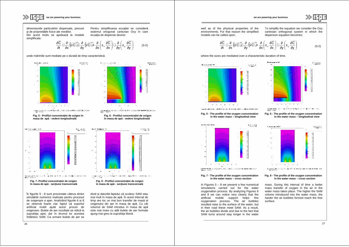
Pentru simplificarea ecuației se considerăsistemul ortogonal cartezian Oxy în care ecuația de dispersie devine:
( ) ( )
∂∂ε
∂∂+
∂∂ε
∂∂=
∂∂+
∂∂+
∂∂
yC
yxC
xCv
yCu
xtC
yx (3-2)
unde mărimile sunt mediate pe o durată de timp caracteristică.
Fig. 5 - Profilul concentra ției de oxigen în masa de ap ă - vedere longitudinal ă
Fig. 6 - Profilul concentra ției de oxigen în masa de ap ă - vedere longitudinal ă
Fig. 7- Profilul concentra ției de oxigen în masa de ap ă - sec țiune transversal ă
Fig. 8 - Profilul concentra ției de oxigen în masa de ap ă - sec țiune transversal ă
În figurile 5 - 8 sunt prezentate câteva dintre simulările numerice realizate pentru procesul de oxigenare a apei. Analizând figurile 6 și 8 se observă foarte clar faptul că suportul artificial mobil ajută acest proces de oxigenare. Bulele de aer rezultate se ridică la suprafața apei, dar în drumul lor acestea întâlnesc SAM. Ca urmare bulele de aer se
divid și datorită faptului că ocolesc SAM stau mai mult în masa de apă. În acest interval de timp are loc un mai bun transfer de masă al oxigenului din aer în masa de apă. Cu cât volumul de SAM introdus în masa de apăeste mai mare cu atât bulele de aer formate ajung mai greu la suprafața liberă.
26
we are powering your business
well as of the physical properties of the environments. For that reason the simplified models can be called upon.
To simplify the equation we consider the Oxy cartesian orthogonal system in which the dispersion equation becomes:
( ) ( )
∂∂ε
∂∂+
∂∂ε
∂∂=
∂∂+
∂∂+
∂∂
yC
yxC
xCv
yCu
xtC
yx (3-2)
where the sizes are mediated over a characteristic duration of time.
Fig. 5 - The profile of the oxygen concentration Fig. 6 - The profile of the oxygen concentrat ion in the water mass – longitudinal view in the water mass – longit udinal view
Fig. 7 - The profile of the oxygen concentration Fig. 8 - The profile of the oxygen concentrat ion in the water mass – cross section in the water mass – cros s section
In Figures 5 – 8 we present a few numerical simulations carried out for the water oxygenation process. By analyzing Figures 6 and 8 we can notice very clearly that the artificial mobile support helps this oxygenation process. The air bubbles resulted raise to the surface of the water, but in their road these meet SAM. As a result, the air bubbles divide and due to the fact that SAM turns around stay longer in the water
mass. During this interval of time a better mass transfer of oxygen in the air in the water mass takes place. The higher the SAM volume introduced into the water mass, the harder the air bubbles formed reach the free surface.
27
we are powering your business
4. Determinarea, pe cale experimental ă, a concentra ţiei de oxigen dizolvat
Măsurătorile s-au efectuat pe acelaşi bazin pentru care s-au realizat modelările matematice şi simulările numerice descrise în capitolul 3 (bazin cu lungimea şi înălţimea de 2 m şi lăţimea de 1 m). Pentru determinarea concentraţiei de oxigen dizolvat în masa de apă s-au utilizat senzori de tip optic conectaţi la un controler ce permite stocarea valorilor înregistrate (oxigen dizolvat, temperatură, dată, oră) şi transmiterea acestora către un calculator. Senzorul situat în capac este acoperit cu un material fluorescent ce este luminat de un LED. Substanţa chimică fluorescentă devine instantaneu excitată şi apoi, pe măsură ce aceasta se relaxează emite o lumină de culoare roşie. Lumina roşie este detectatăde o fotodiodă, iar timpul necesar substanţei chimice să revină la o stare de relaxare este măsurat. La creşterea concentraţiei de oxigen lumina roşie emisă de senzor este redusă şi timpul necesar substanţei fluorescente pentru revenirea la starea de relaxare este mult mai scurt. Determinarea curbelor de oxigenare s-a realizat prin metoda regimului tranzitoriu la variaţia concentraţiei oxigenului dizolvat în masa de apă. Principiul metodei constă în măsurarea vitezei de oxigenare a apei curate începând de la un conţinut nul de oxigen până la concentraţia la saturaţie. Concentraţia la zero a oxigenului s-a reglat prin adăugarea în exces a sulfitului de sodiu în prezenţa ionilor de cobalt, pentru consumarea oxigenului dizolvat din apa iniţială. Excesul de sulfit de sodiu, maxim 10 - 20%, se consumă prin introducerea unei cantităţi de oxigen, considerând drept
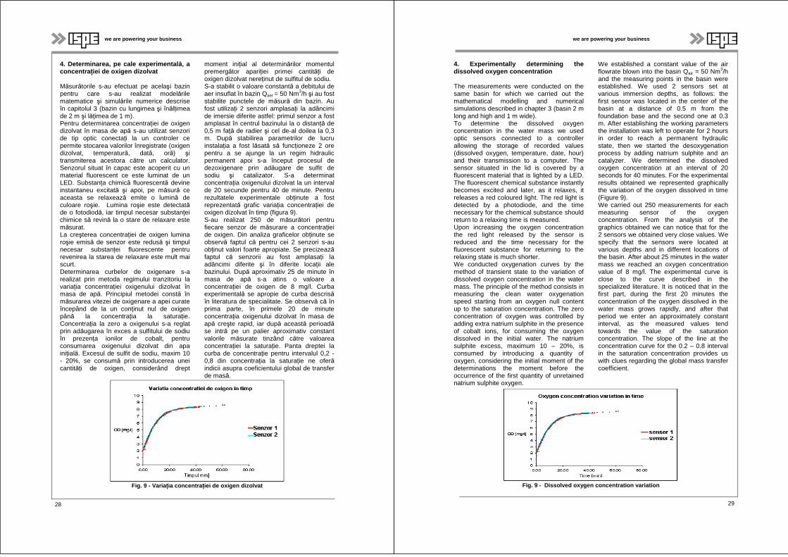
moment iniţial al determinărilor momentul premergător apariţiei primei cantităţi de oxigen dizolvat nereţinut de sulfitul de sodiu. S-a stabilit o valoare constantă a debitului de aer insuflat în bazin Qaer = 50 Nm3/h şi au fost stabilite punctele de măsură din bazin. Au fost utilizați 2 senzori amplasaţi la adâncimi de imersie diferite astfel: primul senzor a fost amplasat în centrul bazinului la o distanţă de 0,5 m faţă de radier şi cel de-al doilea la 0,3 m. După stabilirea parametrilor de lucru instalaţia a fost lăsată să funcţioneze 2 ore pentru a se ajunge la un regim hidraulic permanent apoi s-a început procesul de dezoxigenare prin adăugare de sulfit de sodiu şi catalizator. S-a determinat concentraţia oxigenului dizolvat la un interval de 20 secunde pentru 40 de minute. Pentru rezultatele experimentale obţinute a fost reprezentată grafic variaţia concentraţiei de oxigen dizolvat în timp (figura 9). S-au realizat 250 de măsurători pentru fiecare senzor de măsurare a concentraţiei de oxigen. Din analiza graficelor obţinute se observă faptul că pentru cei 2 senzori s-au obţinut valori foarte apropiate. Se precizeazăfaptul că senzorii au fost amplasaţi la adâncimi diferite şi în diferite locaţii ale bazinului. După aproximativ 25 de minute în masa de apă s-a atins o valoare a concentraţiei de oxigen de 8 mg/l. Curba experimentală se apropie de curba descrisăîn literatura de specialitate. Se observă că în prima parte, în primele 20 de minute concentraţia oxigenului dizolvat în masa de apă creşte rapid, iar după această perioadăse intră pe un palier aproximativ constant valorile măsurate tinzând către valoarea concentraţiei la saturaţie. Panta dreptei la curba de concentraţie pentru intervalul 0,2 - 0,8 din concentraţia la saturaţie ne oferăindicii asupra coeficientului global de transfer de masă.
Fig. 9 - Varia ţia concentra ţiei de oxigen dizolvat
26 28 28
we are powering your business
4. Experimentally determining the dissolved oxygen concentration
The measurements were conducted on the same basin for which we carried out the mathematical modelling and numerical simulations described in chapter 3 (basin 2 m long and high and 1 m wide). To determine the dissolved oxygen concentration in the water mass we used optic sensors connected to a controller allowing the storage of recorded values (dissolved oxygen, temperature, date, hour) and their transmission to a computer. The sensor situated in the lid is covered by a fluorescent material that is lighted by a LED. The fluorescent chemical substance instantly becomes excited and later, as it relaxes, it releases a red coloured light. The red light is detected by a photodiode, and the time necessary for the chemical substance should return to a relaxing time is measured. Upon increasing the oxygen concentration the red light released by the sensor is reduced and the time necessary for the fluorescent substance for returning to the relaxing state is much shorter. We conducted oxygenation curves by the method of transient state to the variation of dissolved oxygen concentration in the water mass. The principle of the method consists in measuring the clean water oxygenation speed starting from an oxygen null content up to the saturation concentration. The zero concentration of oxygen was controlled by adding extra natrium sulphite in the presence of cobalt ions, for consuming the oxygen dissolved in the initial water. The natrium sulphite excess, maximum 10 – 20%, is consumed by introducing a quantity of oxygen, considering the initial moment of the determinations the moment before the occurrence of the first quantity of unretained natrium sulphite oxygen.
We established a constant value of the air flowrate blown into the basin Qair = 50 Nm3/h and the measuring points in the basin were established. We used 2 sensors set at various immersion depths, as follows: the first sensor was located in the center of the basin at a distance of 0.5 m from the foundation base and the second one at 0.3 m. After establishing the working parameters the installation was left to operate for 2 hours in order to reach a permanent hydraulic state, then we started the desoxygenation process by adding natrium sulphite and an catalyzer. We determined the dissolved oxygen concentration at an interval of 20 seconds for 40 minutes. For the experimental results obtained we represented graphically the variation of the oxygen dissolved in time (Figure 9). We carried out 250 measurements for each measuring sensor of the oxygen concentration. From the analysis of the graphics obtained we can notice that for the 2 sensors we obtained very close values. We specify that the sensors were located at various depths and in different locations of the basin. After about 25 minutes in the water mass we reached an oxygen concentration value of 8 mg/l. The experimental curve is close to the curve described in the specialized literature. It is noticed that in the first part, during the first 20 minutes the concentration of the oxygen dissolved in the water mass grows rapidly, and after that period we enter an approximately constant interval, as the measured values tend towards the value of the saturation concentration. The slope of the line at the concentration curve for the 0.2 – 0.8 interval in the saturation concentration provides us with clues regarding the global mass transfer coefficient.
Fig. 9 - Dissolved oxygen concentration variation
29
we are powering your business
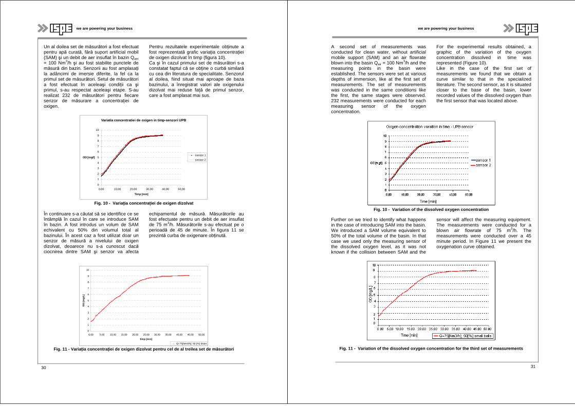
Un al doilea set de măsurători a fost efectuat pentru apă curată, fără suport artificial mobil (SAM) şi un debit de aer insuflat în bazin Qaer
= 100 Nm3/h şi au fost stabilite punctele de măsură din bazin. Senzorii au fost amplasaţi la adâncimi de imersie diferite, la fel ca la primul set de măsurători. Setul de măsurători a fost efectuat în aceleaşi condiţii ca şi primul, s-au respectat aceleaşi etape. S-au realizat 232 de măsurători pentru fiecare senzor de măsurare a concentraţiei de oxigen.
Pentru rezultatele experimentale obţinute a fost reprezentată grafic variaţia concentraţiei de oxigen dizolvat în timp (figura 10). Ca şi în cazul primului set de măsurători s-a constatat faptul că se obţine o curbă similarăcu cea din literatura de specialitate. Senzorul al doilea, fiind situat mai aproape de baza bazinului, a înregistrat valori ale oxigenului dizolvat mai reduse faţă de primul senzor, care a fost amplasat mai sus.
Variatia concentratiei de oxigen in timp-senzori UPB
0
1
2
3
4
5
6
7
8
9
10
0,00 10,00 20,00 30,00 40,00 50,00
Timp [min]
OD [mg/l]senzor 1
senzor 2
Fig. 10 - Varia ţia concentra ţiei de oxigen dizolvat
În continuare s-a căutat să se identifice ce se întâmplă în cazul în care se introduce SAM în bazin. A fost introdus un volum de SAM echivalent cu 50% din volumul total al bazinului. În acest caz a fost utilizat doar un senzor de măsură a nivelului de oxigen dizolvat, deoarece nu s-a cunoscut dacăciocnirea dintre SAM şi senzor va afecta
echipamentul de măsură. Măsurătorile au fost efectuate pentru un debit de aer insuflat de 75 m3/h. Măsurătorile s-au efectuat pe o perioadă de 45 de minute. În figura 11 se prezintă curba de oxigenare obţinută.
0
1
2
3
4
5
6
7
8
9
10
0,00 5,00 10,00 15,00 20,00 25,00 30,00 35,00 40,00 45,00 50,00
timp [min]
OD
[mg/
L]
Q=75[Nm3/h]; 50 [%] bilute
Fig. 11 - Varia ţia concentra ţiei de oxigen dizolvat pentru cel de al treilea set de măsurători
30
we are powering your business
A second set of measurements was conducted for clean water, without artificial mobile support (SAM) and an air flowrate blown into the basin Qair = 100 Nm3/h and the measuring points in the basin were established. The sensors were set at various depths of immersion, like at the first set of measurements. The set of measurements was conducted in the same conditions like the first, the same stages were observed. 232 measurements were conducted for each measuring sensor of the oxygen concentration.
For the experimental results obtained, a graphic of the variation of the oxygen concentration dissolved in time was represented (Figure 10). Like in the case of the first set of measurements we found that we obtain a curve similar to that in the specialized literature. The second sensor, as it is situated closer to the base of the basin, lower recorded values of the dissolved oxygen than the first sensor that was located above.
Fig. 10 - Variation of the dissolved oxygen concent ration
Further on we tried to identify what happens in the case of introducing SAM into the basin. We introduced a SAM volume equivalent to 50% of the total volume of the basin. In that case we used only the measuring sensor of the dissolved oxygen level, as it was not known if the collision between SAM and the
sensor will affect the measuring equipment. The measurements were conducted for a blown air flowrate of 75 m3/h. The measurements were conducted over a 45 minute period. In Figure 11 we present the oxygenation curve obtained.
Fig. 11 - Variation of the dissolved oxygen concent ration for the third set of measurements
31
we are powering your business
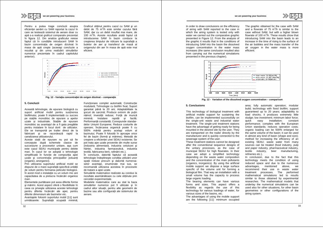
Pentru a putea trage concluzii asupra eficienţei aerării cu SAM raportat la cazul în care se testează sistemul de aerare doar cu apă s-a realizat graficul comparativ prezentat în figura 12. Din analiza graficului reiese faptul că în condiţiile introducerii SAM în bazin concentraţia de oxigen dizolvat în masa de apă creşte (aceeaşi concluzie a rezultat şi din urma realizării simulărilor numerice prezentate în cadrul capitolului anterior).
Graficul obţinut pentru cazul cu SAM şi un debit de 75 m3/h este similar cazului fărăSAM, dar cu un debit insuflat mai mare, de 100 m3/h. Aceste rezultate arată faptul căintroducerea SAM în bazin conduce la creşterea timpului de ridicare la suprafaţă a bulelor de aer şi transferul de masă al oxigenului din aer în masa de apă este mai eficient.
0
1
2
3
4
5
6
7
8
9
10
0,00 10,00 20,00 30,00 40,00 50,00 60,00 70,00
timp [min]
OD
[mg/
L] apa curata; Q=50[Nm3/h]
apa curata; Q=100 [Nm3/h]
bilute; Q=75[Nm3/h]
Fig. 12 - Varia ţia concentra ţiei de oxigen dizolvat – compara ţie
5. Concluzii
Această tehnologie, de epurare biologică cu suport artificial mobil pentru susținerea biofilmului, poate fi implementată cu succes pe stațiile monobloc de epurare a apelor uzate și industriale. Staţiile de epurare monobloc au avantajul de a fi gata pregătite pentru instalare în locul dorit de utilizator. Ele se transportă pe trailer direct de la fabricant şi se racordează rapid la canalizarea utilizatorului. Aceste staţii de epurare nu pot să fie concepute după schemele clasice de succesiune a proceselor unitare, aşa cum este cazul SEAU municipale pentru debite mari. În cazul lor se adoptă o tehnologie simplificată în funcţie de compoziţia apei uzate şi concentraţia principalilor poluanţi (organici, anorganici). Prin utilizarea suportului artificial mobil se dispune de o mare suprafaţă specifică unităţii de volum pentru formarea peliculei biologice. În acest mod o instalaţie cu un volum mic are capacitatea de a prelucra încărcări organice mari. Elementele purtătoare pot avea diferite forme şi mărimi. Acest aspect oferă o flexibilitate în ceea ce priveşte utilizarea acestei tehnologii pentru diferite încărcări ale apei, pentru diferite dimensiuni ale bazinelor etc. Avantajele folosirii suportului mobil [11] sunt următoarele: Suprafaţă ocupată minimă;
Funcţionare complet automată; Construcţie modulară; Tehnologie cu biofilm fixat; Suport garantat până la 20 ani; Adaptabilitate la şocuri de sarcină; Produce extrem de puţin nămol; Investiţii reduse; Forţă de muncăminimă; Instalare rapidă și facilă; Performanţă constantă; Corespunde standar-delor Uniunii Europene; Reduce costurile de operare; Încărcarea organică poate fi cu 500% mărită pentru acelaşi volum al bazinului; Poate fi folosită în aproape orice fel de bazin (formă şi mărime); Metodă de creştere a eficienţei unei SEAU existente; Se pot trata ape uzate provenite din multe surse (industria alimentară, industria celulozei şi hârtiei, industria farmaceutică, industria textilă, fabricarea berii, rafinării etc.). În concluzie, datorită faptului că aceastătehnologie îndeplineşte condiţia utilizării unor spaţii reduse precum şi datorită numeroa-selor avantaje, enumerate mai sus, se recomandă utilizarea acesteia în procesele de tratare a apei uzate. Simulările matematice realizate au condus la rezultate asemănătoare cu cele obţinute prin cercetări experimentale. Modelele matematice care au stat la baza simulărilor numerice pot fi utilizate și în cadrul altor situații, pentru alte geometrii de bazine sau alte configurații ale sistemului de aerare.
32
we are powering your business
In order to draw conclusions on the efficiency of airing with SAM reported to the case in which the airing system is tested only with water we carried out the comparative graphic presented in Figure 12. From the analysis of the graphic it results that in the conditions of introducing SAM into the basin the dissolved oxygen concentration in the water mass increases (the same conclusion resulted also from carrying out the numerical simulations presented in the previous chapter).
The graphic obtained for the case with SAM and a flowrate of 75 m3/h is similar to the case without SAM, but with a higher blown flowrate of 100 m3/h. These results show that introducing SAM into the basin leads to an increase in the time of rising to the surface of the air bubbles and the mass transfer of the air oxygen in the water mass is more efficient.
Fig. 12 - Variation of the dissolved oxygen concent ration – comparison
5. Conclusions
This technology of biological treatment with artificial mobile support for sustaining the biofilm, can be implemented successfully on the single-unit waste and industrial water treatment. The single-unit treatment stations have the advantage of getting ready for being mounted in the desired site by the user. They are transported on the trailer directly by the manufacturer and is quickly connected to the sewerage system of the user. These treatment stations cannot be designed after the conventional sequence designs of the unitary processes, as the case of municipal SEAU for high flowrates. In their case we adopt a simplified technology depending on the waste water composition and the concentration of the main pollutants (organics, inorganics). By using the artificial mobile support we dispose a large surface specific of the volume unit for forming a biological film. That way an installation with a small volume has the capacity to process large organic loading. The bearing elements can have various forms and sizes. This aspect offers a flexibility as regards the use of this technology for various loadings of water, for various sizes of the basins, etc. The advantages of using the mobile support are the following [11]: minimum occupied
area; fully automatic operation; modular build; technology with fixed biofilm; support guaranteed up to 20 years; adaptability to load shocks; it produces extremely little sludge; low investment; minimum labor force; quick easy installation; constant performance; complies with the European Union standards; reduces operation costs; organic loading can be 500% enlarged for the same volume of the basin; it can be used in almost any kind of basin (shape and size); method for increasing the efficiency of an existing SEAU; waste water from many sources can be treated (food industry, pulp and paper industry, pharmaceutical industry, textile industry, beer manufacturing, refineries etc.). In conclusion, due to the fact that this technology meets the condition of using reduced space and due to the numerous advantages, mentioned above, we recommend their use in waste water treatment processes. The performed mathematical simulations led to results similar to those obtained by experimental researches. The mathematical models that underlay the numerical simulations can be used also for other situations, for other basin geometries or other configurations of the airing system.
33
we are powering your business
Bibliografie
1] www.wikipedia.com
[2] http://createchaqua.s-11.dk
[3] http://www.mbbr-media.com
[4] http://www.psiprocess.com
[5] www.alibaba.com
[6] http://www.rvtpe.de
[7] Robescu Di. - Modelarea proceselor biologice de epurare a apelor uzate, Editura Politehnica Press, 2009;
[8] Robescu D. N., Lanyi S., Robescu D., Constantinescu I. - Tehnologii, instalaţii și echipamente epurare, Editura Tehnica, Bucureşti, 2000;
[9] Moga I.C., Năsărîmbă Grecescu B. - Determinarea concentrației de oxigen dizolvat din cadrul unui bioreactor de tip MBBR, Simpozion Internaţional SIMI 2011, Mediu şi Industria, vol.1, ISSN 1843-5831;
[10] Metcalf and Eddy, Inc. - Wastewater Engineering: Treatment and Reuse, fourth edition. New York: McGraw-Hil”, 2003;
[11] Odegaard, H., Rusten, B., Westrum, T., - A new moving bed biofilm reactor - applications and results, „Water Sci. Technol.” 29 (10–11), 1994, pg. 157–165;
Referent:
Consilier tehnico-econ omic ing. Veronica Petri
34
we are powering your business
References
[1] www.wikipedia.com
[2] http://createchaqua.s-11.dk
[3] http://www.mbbr-media.com
[4] http://www.psiprocess.com
[5] www.alibaba.com
[6] http://www.rvtpe.de
[7] Robescu Di. - Modelarea proceselor biologice de epurare a apelor uzate, Editura Politehnica Press, 2009
[8] Robescu D. N., Lanyi S., Robescu D., Constantinescu I. - Tehnologii, instalaţii și echipamente epurare, Editura Tehnica, Bucureşti, 2000
[9] Moga I.C., Năsărîmbă Grecescu B. - Determinarea concentrației de oxigen dizolvat din cadrul unui bioreactor de tip MBBR, Simpozion Internaţional SIMI 2011, Mediu şi Industria, vol. 1, ISSN 1843-5831
[10] Metcalf and Eddy, Inc. - Wastewater Engineering: Treatment and Reuse, fourth edition. New York: McGraw-Hil”, 2003
[11] Odegaard, H., Rusten, B., Westrum, T., - A new moving bed biofilm reactor—applications and results, „Water Sci. Technol.” 29 (10–11), 1994, pg. 157–165;
Reviewer: Technico-economic counsellor eng. Veronica Petri
35
we are powering your business
MODUL ÎN CARE CARACTERISTICILE STATICE DE SARCIN Ă INFLUENŢEAZĂREZULTATELE CALCULELOR REGIMULUI STA ŢIONAR
Nicoleta Elena RO ŞCA1
Rezumat: În articol sunt prezentate metodele practice de determinare a caracteristicilor de sarcină la nivelul sistemului electroenergetic naţional. Dacă metoda analitică are la bazăcaracteristicile statice ale fiecărui receptor conectat în nodul de reţea considerat, caracteristici determinate pe baza condiţiilor de stare electromagnetică, conform modelului matematic (schema echivalentă), metoda experimentală permite, obţinerea funcţiilor P=f(U) şi Q=g(U) pentru un nod de sarcină dat, fără studierea componentei sarcinii şi a parametrilor utilizatorilor. Sunt evidenţiate avantajele şi dezavantajele utilizării fiecărei metode. Pentru a evalua importanţa considerării caracteristicii statice a sarcinii în studiul regimurilor staţionare s-a procedat la analiza unei zone reale a sistemului electroenergetic
naţional, în care consumul a fost modelat considerând două tipuri de caracteristică de sarcină, determinate prin măsurători în cadrul sistemului electroenergetic naţional. Pe baza analizei impactului utilizării caracteristicilor de sarcină P = f(U) şi Q=g(U) se evidenţiază importanţa considerării acesteia în determinarea pierderilor de putere activă în reţele, atât la nivelul zonei de sistem analizate, cât şi la nivelul SEN. De asemenea se prezintă influenţa reglării tensiunii în cadrul benzii admisibile asupra puterii active şi reactive consumate în funcţie de caracteristica de sarcină considerată. Se analizează variaţia puterii active, respectiv reactive în funcţie de variaţia de
tensiuneP
U
∆∆ , respectiv
Q
U
∆∆ .
Cuvinte cheie: metoda analitic ă de calcul, metoda experimental ă, caracteristica de sarcin ă, nivel de tensiune, pierderi de putere activ ă
1. Introducere
Cunoaşterea caracteristicilor statice de sarcină este importantă în:
exploatare: • pentru reglarea corectă în regim staţionar a tensiunii (în special comutarea ploturilor transformatoarelor 110/MT care se realizează în sarcină); • pentru determinarea limitei minime de putere reactivă şi stabilirea DASU (noduri şi valori); • pentru determinarea corectă (prin postcalcul sau/şi prognoză) a pierderilor în reţele.
studii şi proiectare: • pentru calculele de regim staţionar şi prin caracteristicile ei statice; • pentru determinarea mijloacelor de reglaj a tensiunii şi de îmbunătăţire a factorului de putere; • pentru analiza stabilităţii (în principal a stabilităţii de tensiune) – pe timp scurt, mediu şi lung.
Deşi deosebit de importante, în practica curentă actuală nu este uzuală considerarea sarcinii prin caracteristicile ei statice. În acest referat se doreşte sensibilizarea inginerilor energeticieni pentru adoptarea acesteia.
2. Metode practice de determinare a caracteristicilor de sarcin ăă
Pentru determinarea caracteristicilor statice (CS) există – teoretic – două metode:
• metoda analitică de calcul • metoda experimentală.
Metoda analitică are la bază caracteristicile statice ale fiecărui receptor conectat în nodul de reţea considerat, caracteristici determinate pe baza condiţiilor de stare electromagnetică, conform modelului matematic (schema echivalentă).
1 Dr.ing., Secţia Sisteme Energetice, Institutul de Studii şi Proiectări Energetice – I.S.P.E. S.A.
36
we are powering your business
HOW STATIC LOAD CHARACTERISTICS INFLUENCE THE RESUL TS OF STEADY STATE CALCULATIONS
Nicoleta Elena ROŞCA 1
Abstarct: The paper presents the practical method to determine the load characteristics at the level of the National Power System. If the analytical method is based on static characteristics of each receiver connected in the network node considered, characteristics determined on the basis of the electromagnetic state conditions, according to the mathematical model (equivalent diagram), the experimental method allows, obtaining the functions P=f(U) and Q=g(U) for a given load node, without studying the components of the load and the parameters of the users. The advantages and disadvantages of using each method is pointed out. In order to evaluate the importance of considering the static load characteristics in the study on steady states we set out to analyze the real area of the National Power System, in which the consumption was
modeled by considering two types of load characteristics determined by measurements within the National Power System. Based on the analysis of the impact of using the load characteristics P = f(U) and Q=g(U) the author points out the importance of considering it upon determining the active power losses in the networks, both at the level of the system area analyzed, and at the level of the NPS. At the same time the author presents the influence of voltage control within the allowed band on the active and reactive power consumed depending on the load characteristic considered. We analyze the variation of active power, respectively the reactive power, the voltage
variation P
U
∆∆ , respectively
Q
U
∆∆ .
Key words: analytical calculating method, experime ntal method, load characteristic, voltage level, active power losses
1. Introduction
Knowing the static load characteristics is important in:
operation:• for the correct regulation in steady state of voltage (especially switching 110/MV transformer plots that are performed in load); • for determining the minimum reactive power limit and establishing DASU (nodes and values); • for correctly determining (by post-calculation or/and forecast) of losses in the networks.
studies and design: • for the steady state and sizing calculations. In this paper we wish to raise the awareness of energy engineers for adopting this sizing; • for determining the voltage control means and power factor improvement;
• for stability analysis (mainly voltage stability) – on short, mid and long term. Although very important, in current practice it is not usual to consider the load by its static characteristics. In this paper we wish to raise the awareness of energy engineers for adopting it.
2. Practical methods for determining the load characteristics
For determining the static characteristics (SC) there are – theoretically – two methods:
• the analytical calculation method • the experimental method.
The analytical method is based on the static characteristics of each receiver connected to the considered network, characteristics determined based on the electromagnetic state conditions according to the mathematical diagram (equivalent diagram).
2Ph.D., Eng., Power Systems Division, Institute for Studies and Power Engineering - ISPE SA
35 37
we are powering your business
Metoda analitică se bazează pe cunoaşterea caracteristicilor nodului şi a consumului (P şi Q) al fiecărui receptor la tensiunea nominală. Se alcătuieşte schema echivalentă de modelare a întregului consum la puterea nominală, după care trebuie să se determine dependenţa consumului de putere activă şi reactivă cu tensiunea. Este evident că este dificil de determinat şi schema corectă a totalităţii componentelor consumului din nod, regimul simultan al acestora şi mai ales comportarea ansamblului la variaţiile de tensiune. S-a stabilit că limitele de variaţie a P şi Q pentru o variaţie a tensiunii în limitele (0,9 – 1,1)Un se poate exprima printr-o relaţie polinomială de gradul 2.
P = P0 (p0 + p1ku + p2k2
u) (1) Q = Q0 (q0 + q1ku + q2k
2u)
p0, p1, p2, q0, q1, q2 fiind factori de aproximare
şi
NUu
Uk = .
În final este necesară stabilirea factorilor pe baza unor rezultate obţinute experimental, aplicând metoda celor mai mici pătrate.
Metoda experimentală permite, pe de o parte obţinerea funcţiilor P=f(U) şi Q=g(U) pentru nodul de sarcină concret, fără studierea conţinutului şi parametrilor consumatorilor, iar pe de altă parte, exactitatea caracteristicii statice obţinute prin metoda aceasta este mai bună decât prin metoda analitică din cauza dificultăţilor luării în considerare în ultimul caz a unor astfel de factori ca puterea de magnetizare a transformatoarelor şi motoarelor, existenţa instalaţiilor de compensare a puterii reactive ş.a.m.d. Determinarea experimentală a caracteristicii statice (CS) se poate realiza prin metoda experimentului activ sau pasiv. Metoda experimentului activ oferă cele mai precise rezultate la determinarea CS. Esenţa efectuării experimentului activ constăîn următoarele: Schimbând deliberat tensi-unea la bornele obiectului de studiu (fie motor asincron, sarcină statică sau nod de sarcină) sau într-un nod al reţelei cu ajutorul mijloacelor cunoscute de reglare a tensiunii (de excitare a generatoarelor, compensa-toarelor sincrone, sau prin schimbarea
ploturilor transformatorului sub sarcină) se determină dependenţele P=f(U) şi Q=g(U). Măsurătorile se efectuează într-o perioadă în care sarcina în nod se menţine practic constantă. Aceasta necesită o analizăprealabilă pentru mai multe zile a curbei de sarcină din nodul respectiv. Se realizează în funcţie de posibilităţi modificarea nivelului de tensiune. Perioada în care consumul de energie electrică este practic staţionar se determinăprin cercetarea statistică a curbelor tipice de sarcină (pentru zilele de lucru şi cele de sărbători) în mijlocul schimbului de lucru (începutul şi sfârşitul schimburilor se exclude). Apoi se analizează rezultatele cercetărilor efectuate, cu scopul evitării erorilor introduse de eventualele variaţii de sarcină apărute şi se efectuează prelucrarea datelor prin metodele matematicii statistice pentru obţinerea unei valori medii. Prin aproximarea ulterioară a CS obţinute şi prin examinarea erorilor obţinute în rezultatul aproximării, se finalizează metoda experimentului activ. Utilizarea metodei experimentului activ este limitată din următoarele cauze: - experimentul activ întotdeauna este legat de intervenţia în procesul de funcţionare normală a unor variaţii de sarcină, ceea ce, într-o oarecare măsură, reduce gradul de fiabilitate al rezultatelor; - dificultatea reglării tensiunii într-un domeniu necesar pentru nodurile de sarcină puternice, deoarece valoarea relativă a abaterii sarcinii este invers proporţională cu puterea din nodul de sarcină; - imposibilitatea obţinerii CS pentru toate regimurile necesare ale nodului de sarcină; - necesitatea excluderii la construirea CS a variaţiei sarcinii şi a tensiunii din cauze tehnologice pentru excluderea erorilor considerabile. În metoda experimentului pasiv, pentru obţinerea efectului regulator al sarcinii se utilizează abaterile mici şi întâmplătoare ale tensiunii, existente real în orice reţea. Deci abaterile de tensiune există ca prototip al variaţiei tensiunii realizată dorit, în cazul experimentului activ. În cazul dat, se creeazăşi se înregistrează abateri ale puterilor activă∆P şi reactivă ∆Q – ca reacţie a nodului de sarcină la excitările externe ale sistemului. Măsurând valorile medii pentru un anumit interval de timp ∆U, ∆P, ∆Q, se determinăefectele reglatoare ale puterii active KP = ∆P/ ∆U şi ale puterii reactive KQ = ∆Q / ∆U. Numeric valorile ∆P, ∆Q, ∆U constituie circa
36 38
we are powering your business
The analytical method is based on the knowledge of the characteristics of the node and consumption (P and Q) of each receiver at rated voltage. We make up the equivalent modelling diagram of the entire consumption at rated power, then the dependence of the active and reactive power consumption with the voltage is determined. It is obvious that it is difficult to determine also the correct diagram of all the components of the consumption in the node, their simultaneous state and especially the behavior of the assemblage at voltage variations. It was established that the variation limits of P and Q for a voltage variation within the range (0.9 – 1.1)Un can be expressed by a polynomial relation of the 2nd degree.
P = P0 (p0 + p1ku + p2k2
u) (1)Q = Q0 (q0 + q1ku + q2k
2u)
p0, p1, p2, q0, q1, q2
being approximation factors
and
NUu
Uk = .
In the end it is necessary to establish the factors based on results obtained experimentally, by applying the method of least squares.
The experimental method allows, on the one hand, to obtain the functions P=f(U) and Q=g(U) for the concrete load node, without studying the content and consumer parameters, and, on the other, the accuracy of the static characteristics obtained by this method is better than by the analytical method because of the difficulties of taking into consideration in the last case of such factors like the magnetizing power of transformers and engines, the existence of reactive power compensation installations a.s.o. The experimental determination of the static characteristic (SC) can be carried out by the method of the active or passive experiment. The active experiment method offers the most accurate results in determining the SC. The essence of conducting the active experiment consists in the following: deliberately changing the voltage at the
terminals of the study object (either asynchronous engine, static load or load node) or in a node of the network by the known voltage control means (of exciting generators, synchronous compensators, or by changing the loaded transformer plots) are determined the dependencies P=f(U) and Q=g(U). The measurements are conducted during a period in which the load in the node is maintained practically constant. That requires a preliminary analysis for several days of the load curve in the respective node. It is carried out according to the possibilities of changing the voltage level. The period in which the electric power consumption is practically determined by the statistical research of the typical load curves (for working days and holidays) in the middle of the work shifts (the beginning and end of shifts are excluded). Then we analyze the results of the researches conducted, in order to avoid the errors introduced by the possible load variations occurred and the data are processed by the statistical mathematics method to obtain an average value. By later approximating the SC obtained and by examining the errors obtained in the result of the approximation, the active experiment method is finalized. The use of the active experiment method is limited for the following causes:
- the active experiment is always related to the intervention in the regular operation process of load variations, which, to a certain extent, reduces the degree of reliability of the results;
- the difficulty of controlling voltage in a range necessary for the strong load nodes, because the relative value of load deviation is inversely proportional to the power in the load node;
- the impossibility of obtaining the SC for all the necessary states of the load node;
- the necessity of excluding, when the SC is built, the load variation and the voltage variation for technological reasons in order to exclude considerable errors. In the passive experiment method, to obtain the regulating effect of the load we use small random deviations of voltage, actually existing in any network. Although the voltage deviations exist as a prototype of voltage variation deliberately carried out, in the case of the active experiment. In the given case, are created and recorded deviations of the active ∆P and reactive ∆Q powers – as a reaction of the load nodes at the external
39
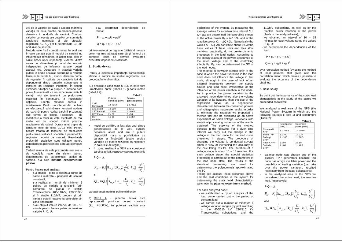
we are powering your business
1% de la valorile de bază a acestor mărimi şi variaţia lor lentă, practic, nu creează procese dinamice în nodurile de sarcină. Conform valorilor cunoscute ale puterilor consumate la tensiunea nominală şi ale efectelor reglatoare KP, KQ, pot fi determinate CS ale nodurilor de sarcină. Metoda este însă corectă numai în acel caz în care variaţia puterii nodului de sarcină nu influenţează tensiunea în acest nod, deci în cazul lipsei unei impedanţe externe dintre sursa de alimentare şi nodul de sarcină, independent de influenţa variaţiei puterii acestui nod. Deoarece în practică variaţia puterii în nodul analizat determină şi variaţia tensiunii la barele lui, atunci utilizarea curbei de regresie, în calitate de caracteristică de dependenţă dintre puterile consumate şi tensiune dă rezultate incorecte. În scopul eliminării situaţiei s-a propus o metodă care poate fi examinată ca un experiment activ la variaţii mici ale tensiunii cu prelucrarea statistică în continuare, a rezultatelor obţinute. Esenţa metodei constă în următoarele. Pentru un interval dat de timp se efectuează schimbarea tensiunii nodului de sarcină pentru curba sarcinii prezentatăsub formă de trepte. Procedura de modificare a tensiunii este efectuată de mai multe ori cu scopul măririi preciziei rezultatelor de calcul. Durata unei trepte de tensiune este de circa 10-15 min. Pentru fiecare treaptă de tensiune, se efectueazăprelucrarea statistică specială a parametrilor regimului nodului de sarcină. Rezultatele prelucrării statistice sunt utilizate pentru determinarea polinoamelor care aproximeazăCS. Ţinând seama de cele prezentate mai sus şi de condiţiile reale din sistem pentru determinarea de caracteristici statice de sarcină, s-a ales metoda experimental ăpasiv ă.
Pentru fiecare nod analizat: - s-a stabilit – printr-o analiză a curbei de
sarcină realizată – perioada de sarcinăconstantă;
- s-a realizat un număr de minimum 5 paliere de variaţie a tensiunii (prin comutare de ploturi în staţiile Transelectrica 400/110kV, 220/110kV şi în staţiile 110/MT, precum şi prin variaţia puterii reactive la centralele din zona analizată);
- s-au obţinut într-un interval de 10 – 15 minute pentru fiecare palier de tensiune valorile P, Q, U;
- s-au determinat dependenţele de forma:
P = p0 + p1U + p2U2
Q = q0 + q1U + q2U2
printr-o metodă de regresie (utilizând metoda celor mai mici pătrate) care dă şi factorul de corelare, ceea ce permite evaluarea exactităţii dependenţei obţinute.
3. Studiu de caz
Pentru a evidenţia importanţa caracteristicii statice a sarcinii în studiul regimurilor s-a procedat în felul următor:
S-a analizat o zonă reală a SEN în care sunt următoarele surse (tabelul 1) şi consumatori (tabelul 2): Tabel 1
Puterea nominală (MW)
Puterea generată (MW)
CNE Cernavodă
1 x 706,6 1 x 706,6
CTE Brăila 1 x 300 1 x 210 CET Barboşi 1 x 100 1 x 66,5 CET Palas 2 x 50 2 x 50 CET Smârdan
1 x 60 1 x 48,2
• nodul de echilibru a fost ales unul dintre
generatoarele de la CTE Turceni deoarece acest nod are o putere disponibilă mare şi posibilitatea de variaţie a încărcării (poate prelua variaţiile de putere rezultate ca necesare în calculele de regim);
• în zona analizată a SEN s-a considerat sarcina activă, respectiv sarcina reactivă:
P,Q = ct.
2
var _ _ _ 2n P S P I P Zn n
U UP P k k k
U U
= ⋅ + ⋅ + ⋅
şi 2
var _ _ _ 2n Q S Q I Q Zn n
U UQ Q k k k
U U
= ⋅ + ⋅ + ⋅
variază după modelul polinomial unde:
a) Cazul A - puterea activă este reprezentată printr-un curent constant ( _ 100%P Ik = ), iar puterea reactivă este
40
we are powering your business
excitations of the system. By measuring the average values for a certain time interval ∆U, ∆P, ∆Q are determined the controlling effects of the active power KP = ∆P / ∆U and of the reactive power KQ = ∆Q / ∆U. Numerically the values ∆P, ∆Q, ∆U constitute about 1% of the basic values of these units and their slow variation, practically, do not create dynamic processes in the load nodes. According to the known values of the powers consumed at the rated voltage and of the controlling effects KP, KQ can be determined the SC of the load nodes. The method is however correct only in the case in which the power variation in the load node does not influence the voltage in that node, although in the case of lack of an external impedance between the supply source and load node, irrespective of the influence of the power variation in this node. As in practice the power variation in the analyzed node determines also the voltage variation at its busbars, then the use of the regression curve, as a dependence characteristic between the consumed powers and voltage gives inaccurate results. In order to eliminate the situation we proposed a method that can be examined as an active experiment at small voltage variations with statistical processing further on, of the results obtained. The essence of the method consists in the following. For a given time interval we carry out the change in the voltage in the load node for the load curve presented in stages. The procedure of changing the voltage is conducted several times in view of increasing the accuracy of the calculating results. The duration of a voltage stage is about 10 – 15 minutes. For each voltage stage, the special statistical processing is carried out of the parameters of the load node state. The results of the statistical processing are used for determining the polynominals approximating the SC. Taking into account those presented above and the real conditions in the system for determining the static load characteristics, we chose the passive experiment method .
For each analyzed node: - we established – by an analysis of the
load curve carried out – the period of constant load;
- we carried out a number of minimum 5 voltage variation ranges (by plot switching in the 400/110 kV, 220/110 kV Transelectrica substations, and the
110/MV substations, as well as by the reactive power variation at the power plants in the analyzed area);
- we obtained an interval of 10 – 15 minutes for each voltage range the values P, Q, U;
- we determined the dependencies of the form:
P = p0 + p1U + p2U2
Q = q0 + q1U + q2U2
by a regression method (by using the method of least squares) that gives also the correlation factor, which makes it possible to evaluate the accuracy of the dependence obtained.
3. Case study
To point out the importance of the static load characteristic in the study of the states we proceeded as follows:
We analyzed a real area of the NPS (the National Power System) in which are the following sources (Table 1) and consumers (Table 2): Table 1
Rated power (MW)
Generated power (MW)
CernavodăNPP 1 x 706.6 1 x 706.6
Brăila TPP 1 x 300 1 x 210 Barboși CHPP
1 x 100 1 x 66.5
Palas CHPP 2 x 50 2 x 50 Smârdan CHPP
1 x 60 1 x 48.2
• balance node was chosen one of the Turceni TPP generators because this node has a high available power and the possibility of loading variation (can take over the power variations resulted necessary from the state calculations);
• in the analyzed area of the NPS we considered the active load, the reactive load, respectively:
P,Q = ct.
2
var _ _ _ 2n P S P I P Zn n
U UP P k k k
U U
= ⋅ + ⋅ + ⋅
and
2
var _ _ _ 2n Q S Q I Q Zn n
U UQ Q k k k
U U
= ⋅ + ⋅ + ⋅
41
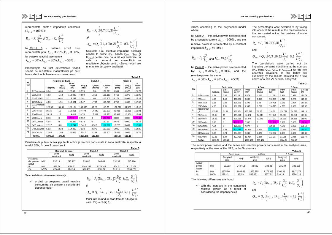
we are powering your business
reprezentată printr-o impedanţă constantă( _ 100%Q Zk = );
var nn
UP P
U= ⋅ şi
2
var 2nn
UQ Q
U= ⋅
b) Cazul B - puterea activă este reprezentată prin: _ _70%, 30%P S P Ik k= = ,
iar puterea reactivă asemenea
_ _ _30%, 20%, 50%Q S Q I Q Zk k k= = = .
Procentajele au fost determinate ţinând seama de rezultatele măsurătorilor pe care le-am efectuat la barele unor consumatori;
var 0,7 0,3nn
UP P
U
= ⋅ + ⋅
şi
2
var 20,3 0, 2 0,5n
n n
U UQ Q
U U
= ⋅ + ⋅ + ⋅
Calculele s-au efectuat impunând aceleaşi condiţii la surse (PG, banda Qmin, Qmax şi Uimpus) pentru cele două situaţii analizate. În cele ce urmează se exemplifică cu rezultatele obţinute pentru câteva noduri ale unei reţele de 110kV analizată:
Tabel 2
Nr.crt
Regimul de baza Cazul A Cazul B
Pct (MW) Qct
(MVAr)
Ucalc_ regim (kV)
P=f(U) (MW)
Q=f(U) (MVAr)
U_recalc (kV)
P=f(U) (MW)
Q=f(U) (MVAr)
U_ recalc (kV)
1 217Nazarcea 3,24 0,86 122,43 3.573 1046 121.291 3.344 0,976 121.79 2 222Liesti 4,63 1,18 118,082 4.889 1.316 116.163 4.718 1,272 116.99 3 228T.Vladi 3,11 0,92 118,298 3,291 1.03 116.405 3.171 0,994 117.22 4 229Schela 4,66 1,51 118,621 4.947 1.702 116.775 4.756 1,638 117.57
6 231Smardan_A 125,96 31,31 120,154 135.533 36.25 118.36 129.098 34,538 119.13
8 235Filiesti 35,15 15 119,011 37.474 17.049 117.273 35.918 16,351 118.01 9 236Filiesti 35,15 15 119,011 3.474 17.049 117.273 35.918 16,351 118.01 29 263Sacele 0,86 0 122,9 0.952 0 121.712 0.889 0,000 122.31 30 264Lumina 4,54 0 121,889 4.974 0 120.51 4.678 0,000 121.13 70 347Urziceni 12,17 3,8 113,741 12.415 3.517 112.212 12.265 3,487 112.87 71 348Cazanes 6,83 2,24 114,838 7.039 2.379 113.363 6.905 2,339 114.00 74 903Ovidiu 12,63 1,84 122,426 13.917 2.234 121.207 13.035 2,086 121.75
TOTAL 1275,56 475,43 1363.355 537.451 1304.31 516,15
Pierderile de putere activă şi puterile active şi reactive consumate în zona analizată, respectiv la nivelul SEN, în cele 3 cazuri sunt:
Tabel 3 Regimul de baza Cazul A Cazul B
Zona analizată
SEN Zona analizată
SEN Zona analizată
SEN
Pierderile de putere activă
MW 23.013 243.413 23.682 248.83 23.239 245.196
Pc MW 1275.56 9088.52 1363.355 9176.313 1304.31 9117.273 Qc MVAr 475.43 3515.4 537.451 3577.52 516.15 3556.222
Se constată următoarele diferenţe:
o dată cu creşterea puterii reactive consumate, ca urmare a considerării dependenţelor
2
var _ _ _ 2n P S P I P Zn n
U UP P k k k
U U
= ⋅ + ⋅ + ⋅
şi
2
var _ _ _ 2n Q S Q I Q Zn n
U UQ Q k k k
U U
= ⋅ + ⋅ + ⋅
tensiunile în noduri scad faţă de situaţia în care P,Q = ct (fig 1);
42 42
we are powering your business
varies according to the polynomial model where:
a) Case A – the active power is represented by a constant current _ 100%P Ik = , and the
reactive power is represented by a constant impedance _ 100%Q Zk = ;
var nn
UP P
U= ⋅ and
2
var 2nn
UQ Q
U= ⋅
b) Case B – the active power is represented by: _ _70%, 30%P S P Ik k= = , and the
reactive power the same
_ _ _30%, 20%, 50%Q S Q I Q Zk k k= = = .
The percentages were determined by taking into account the results of the measurements that we carried out at the busbars of some consumers;
var 0,7 0,3nn
UP P
U
= ⋅ + ⋅
and
2
var 20,3 0, 2 0,5n
n n
U UQ Q
U U
= ⋅ + ⋅ + ⋅
The calculations were carried out by imposing the same conditions at the sources (PG, band Qmin, Qmax şi Uimposed) for the two analyzed situations. In the below we exemplify by the results obtained for a few nodes of a 110 kV network analyzed:
Table 2
No.
Basic state A Case B Case
Pct (MW) Qct (MVAr)
Ucalc_state (kV)
P=f(U) (MW)
Q=f(U) (MVAr)
U_recalc (kV)
P=f(U) (MW)
Q=f(U) (MVAr)
U_recalc (kV)
1 217Nazarcea 3.24 0.86 122.43 3.573 1.046 121.291 3.344 0.976 121.79 2 222Liesti 4.63 1.18 118.082 4.889 1.316 116.163 4.718 1.272 116.99 3 228T.Vladi 3.11 0.92 118.298 3.291 1.03 116.405 3.171 0.994 117.22 4 229Schela 4.66 1.51 118.621 4.947 1.702 116.775 4.756 1.638 117.57
6 231Smardan _A 125.96 31.31 120.154 135.533 36.25 118.36 129.098 34.538 119.13
8 235Filiesti 35.15 15 119.011 37.474 17.049 117.273 35.918 16.351 118.01 9 236Filiesti 35.15 15 119.011 37.474 17.049 117.273 35.918 16.351 118.01 29 263Sacele 0.86 0 122.9 0.952 0 121.712 0.889 0.000 122.31 30 264Lumina 4.54 0 121.889 4.974 0 120.51 4.678 0.000 121.13 70 347Urziceni 12.17 3.38 113.741 12.415 3.517 112.212 12.265 3.487 112.87 71 348Cazanes 6.83 2.24 114.838 7.039 2.379 113.363 6.905 2.339 114.00 74 903Ovidiu 12.63 1.84 122.426 13.917 2.234 121.207 13.035 2.086 121.75
TOTAL 1275.56 475.43 1363.355 537.451 1304.31 516.15
The active power losses and the active and reactive powers consumed in the analyzed area, respectively at the level of the NPS, in the 3 cases are: Table 3
Basic state A Case B Case Analyzed
area NPS Analyzed area NPS Analyzed
area NPS
Active power losses
MW 23.013 243.413 23.682 248.83 23.239 245.196
Pc MW 1275.56 9088.52 1363.355 9176.313 1304.31 9117.273 Qc MVAr 475.43 3515.4 537.451 3577.52 516.15 3556.222
The following differences are found:
with the increase in the consumed reactive power, as a result of considering the dependencies
2
var _ _ _ 2n P S P I P Zn n
U UP P k k k
U U
= ⋅ + ⋅ + ⋅
and
2
var _ _ _ 2n Q S Q I Q Zn n
U UQ Q k k k
U U
= ⋅ + ⋅ + ⋅
43
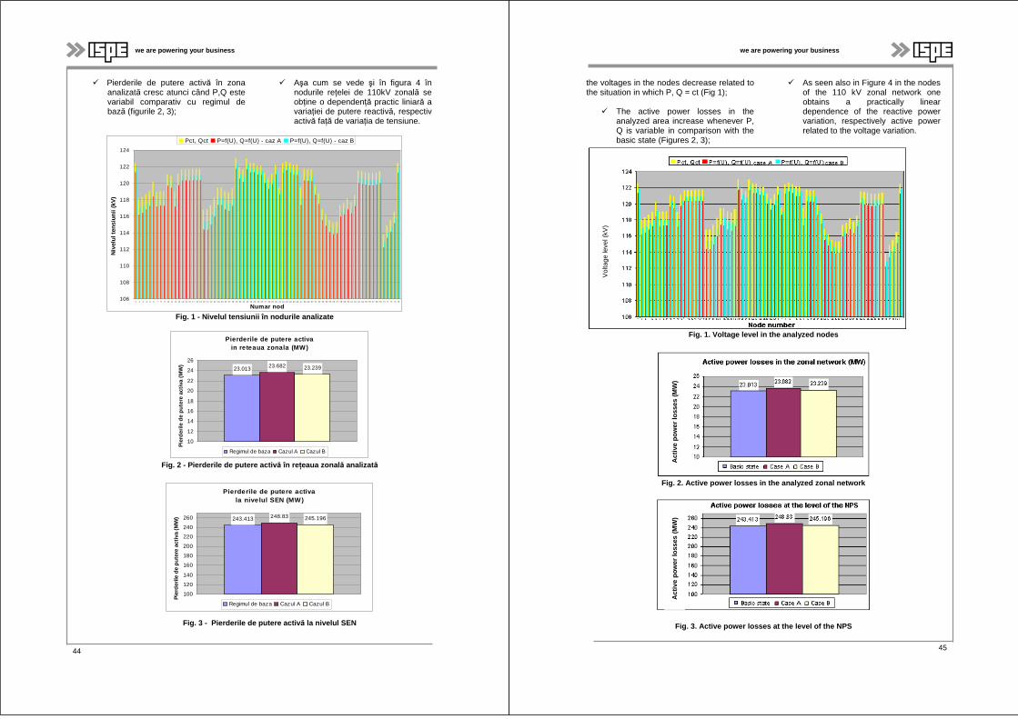
we are powering your business
Pierderile de putere activă în zona analizată cresc atunci când P,Q este variabil comparativ cu regimul de bază (figurile 2, 3);
Aşa cum se vede şi în figura 4 în nodurile reţelei de 110kV zonală se obţine o dependenţă practic liniară a variaţiei de putere reactivă, respectiv activă faţă de variaţia de tensiune.
106
108
110
112
114
116
118
120
122
124
1 2 3 4 5 6 7 8 9 10 11 12 13 14 15 16 17 18 19 20 21 22 23 24 25 26 27 28 29 30 31 32 33 34 35 36 37 38 39 40 41 42 43 44 45 46 47 48 49 50 51 52 53 54 55 56 57 58 59 60 61 62 63 64 65 66 67 68 69 70 71 72 73 74
Numar nod
Niv
elul
tens
iuni
i (kV
)
Pct, Qct P=f(U), Q=f(U) - caz A P=f(U), Q=f(U) - caz B
Fig. 1 - Nivelul tensiunii în nodurile analizate
Pierderile de putere activa in reteaua zonala (MW)
23.013 23.682 23.239
10
12
14
16
18
20
22
24
26
Pie
rder
ile d
e pu
tere
act
iva
(MW
)
Regimul de baza Cazul A Cazul B
Fig. 2 - Pierderile de putere activ ă în re ţeaua zonal ă analizat ă
Pierderile de putere activa la nivelul SEN (MW)
243.413 248.83 245.196
100
120
140
160
180
200
220
240
260
Pie
rder
ile d
e pu
tere
act
iva
(MW
)
Regimul de baza Cazul A Cazul B
Fig. 3 - Pierderile de putere activ ă la nivelul SEN
44
we are powering your business
the voltages in the nodes decrease related to the situation in which P, Q = ct (Fig 1);
The active power losses in the analyzed area increase whenever P, Q is variable in comparison with the basic state (Figures 2, 3);
As seen also in Figure 4 in the nodes of the 110 kV zonal network one obtains a practically linear dependence of the reactive power variation, respectively active power related to the voltage variation.
Fig. 1. Voltage level in the analyzed nodes
Fig. 2. Active power losses in the analyzed zonal n etwork
Fig. 3. Active power losses at the level of the NPS
Vol
tage
leve
l (kV
)
Act
ive
pow
er lo
sses
(M
W)
A
ctiv
e po
wer
loss
es (
MW
)
45
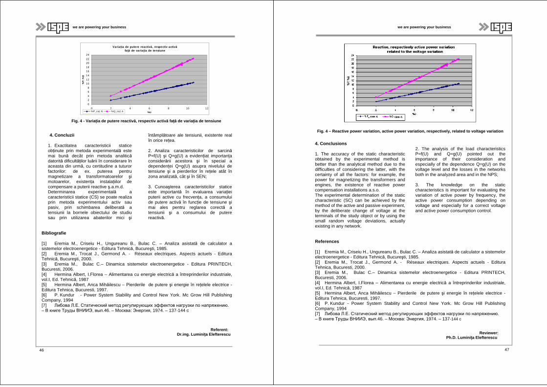
we are powering your business
Varia ţia de putere reactiv ă , respectiv activ ăfa ţă de varia ţia de tensiune
0
2
4
6
8
10
12
14
16
18
20
22
24
0 2 4 6 8 10 12%U
%P
, %Q
%P_caz A %Q_caz A
Fig. 4 - Varia ţia de putere reactiv ă, respectiv activ ă faţă de varia ţia de tensiune
4. Concluzii
1. Exactitatea caracteristicii statice obţinute prin metoda experimentală este mai bună decât prin metoda analiticădatorită dificultăţilor luării în considerare în aceasta din urmă, cu certitudine a tuturor factorilor: de ex. puterea pentru magnetizare a transformatoarelor şi motoarelor, existenţa instalaţiilor de compensare a puterii reactive ş.a.m.d. Determinarea experimentală a caracteristicii statice (CS) se poate realiza prin metoda experimentului activ sau pasiv, prin schimbarea deliberată a tensiunii la bornele obiectului de studiu sau prin utilizarea abaterilor mici şi
întâmplătoare ale tensiunii, existente real în orice reţea.
2. Analiza caracteristicilor de sarcinăP=f(U) şi Q=g(U) a evidenţiat importanţa considerării acestora şi în special a dependenţei Q=g(U) asupra nivelului de tensiune şi a pierderilor în reţele atât în zona analizată, cât şi în SEN;
3. Cunoaşterea caracteristicilor statice este importantă în evaluarea variaţiei puterii active cu frecvenţa, a consumului de putere activă în funcţie de tensiune şi mai ales pentru reglarea corectă a tensiunii şi a consumului de putere reactivă.
Bibliografie
[1] Eremia M., Criseiu H., Ungureanu B., Bulac C. – Analiza asistată de calculator a sistemelor electroenergetice - Editura Tehnică, Bucureşti, 1985. [2] Eremia M., Trocat J., Germond A. - Réseaux electriques. Aspects actuels - Editura Tehnică, Bucureşti, 2000. [3] Eremia M., Bulac C.– Dinamica sistemelor electroenergetice - Editura PRINTECH, Bucuresti, 2006. [4] Hermina Albert, I.Florea – Alimentarea cu energie electrică a întreprinderilor industriale, vol.I, Ed. Tehnică, 1987 [5] Hermina Albert, Anca Mihăilescu – Pierderile de putere şi energie în reţelele electrice - Editura Tehnica, Bucuresti, 1997. [6] P. Kundur - Power System Stability and Control New York. Mc Grow Hill Publishing Company, 1994 [7] Либова Л.Е. Статический метод регулирующих эффектов нагрузки по напряжению. – В книге Труды ВНИИЭ, вып.46. – Москва: Энергия, 1974. – 137-144 с
Referent: Dr.ing. Lumini ţa Elefterescu
44 46
we are powering your business
Fig. 4 – Reactive power variation, active power var iation, respectively, related to voltage variation
4. Conclusions
1. The accuracy of the static characteristic obtained by the experimental method is better than the analytical method due to the difficulties of considering the latter, with the certainty of all the factors: for example, the power for magnetizing the transformers and engines, the existence of reactive power compensation installations a.s.o. The experimental determination of the static characteristic (SC) can be achieved by the method of the active and passive experiment, by the deliberate change of voltage at the terminals of the study object or by using the small random voltage deviations, actually existing in any network.
2. The analysis of the load characteristics P=f(U) and Q=g(U) pointed out the importance of their consideration and especially of the dependence Q=g(U) on the voltage level and the losses in the networks both in the analyzed area and in the NPS;
3. The knowledge on the static characteristics is important for evaluating the variation of active power by frequency, the active power consumption depending on voltage and especially for a correct voltage and active power consumption control.
References
[1] Eremia M., Criseiu H., Ungureanu B., Bulac C. – Analiza asistată de calculator a sistemelor electroenergetice - Editura Tehnică, Bucureşti, 1985. [2] Eremia M., Trocat J., Germond A. - Réseaux electriques. Aspects actuels - Editura Tehnica, Bucuresti, 2000. [3] Eremia M., Bulac C.– Dinamica sistemelor electroenergetice - Editura PRINTECH, Bucuresti, 2006. [4] Hermina Albert, I.Florea – Alimentarea cu energie electrică a întreprinderilor industriale, vol.I, Ed. Tehnică, 1987 [5] Hermina Albert, Anca Mihăilescu – Pierderile de putere şi energie în reţelele electrice - Editura Tehnica, Bucuresti, 1997. [6] P. Kundur - Power System Stability and Control New York. Mc Grow Hill Publishing Company, 1994 [7] Либова Л.Е. Статический метод регулирующих эффектов нагрузки по напряжению. – В книге Труды ВНИИЭ, вып.46. – Москва: Энергия, 1974. – 137-144 с
Reviewer: Ph.D. Lumini ţa Elefterescu
47
we are powering your business
SECURITATEA APROVIZIONĂRII CU ENERGIE A ROMÂNIEI
Irina VODĂ1, Anca Simona BARDICI 2, Roxana IVAN 3, Mihaela BEDREAG Ă3
Rezumat: Energia este o componentă vitalăpentru dezvoltarea economico – socială a României, ceea ce impune adoptarea unei strategii energetice pentru satisfacerea necesarului de energie la un preț cât mai scăzut adecvat unei economii moderne și unui standard de viață civilizat cu respectarea principiilor dezvoltării durabile.
În acest articol se face o analiză a consumului de energie al României și a modului de acoperire a acestuia în perioada 2000 - 2010 pentru a evidenția direcțiile de acțiune pentru asigurarea securității aprovizionării cu energie în condițiile impuse de directivele Uniunii Europene referitoare la energie și mediu.
Cuvinte cheie: consum de energie primar ă, eficien ță energetic ă, energie electric ă, energie nuclear ă, resurse energetice regenerabile.
1. Introducere
Energia este un factor strategic și o componentă vitală pentru dezvoltarea economică şi progresul societăţii în ansamblu generând o serie de preocupări la nivel mondial. Într-o economie din ce în ce mai globalizată, strategia energetică a unei ţări trebuie să ţinăseama de contextul evoluţiilor şi schimbărilor care au loc pe plan mondial.
În ultimii ani, consumul de energie la nivel global a crescut cu un ritm mai mare decât în etapele anterioare, ceea ce atrage atenția căpentru a se atinge durabilitatea în acest domeniu este nevoie ca energia să se producă, să se furnizeze şi să se consume într-un mod mai eficient decât până acum şi cu un impact redus asupra mediului.
Există un consens al diferitelor instituţii internaţionale (WEC, IAEA, IEA, OECD) care estimează că dacă actualele legi şi politici energetice rămân neschimbate până în 2035, cererea mondială de energie va creşte cu aproape 50% comparativ cu anul 2008.
Recesiunea economică globală, care a început în 2007 şi a continuat în 2009, a avut un impact profund pe termen scurt asupra consumului de energie mondial. Acesta s-a redus cu 1,2% în 2008 față de cel al anului 2007 şi cu 2,2% în 2009 față de cel al anului 2008, deoarece industria prelucrătoare a intrat în declin, iar cererea de bunuri şi servicii s-a redus. Este de aşteptat ca, pe măsură ce situaţia economică se îmbunătăţeşte, cele mai multe naţiuni sărevină pe direcţiile de creştere economicăanticipate înainte de începerea recesiunii. Ponderea cea mai mare în creşterea consumului de energie până în 2035 o vor avea ţările din afara Organizaţiei pentru Cooperare Economică şi Dezvoltare* (ţări non - OECD), de 84%, comparativ cu doar 14% pentru ţările OECD.
Din evoluţia consumului mondial al diferitelor forme de energie (figura 1) rezultă că energia nucleară şi combustibilii fosili (combustibilii lichizi, gazul natural şi cărbunele) vor continua să acopere cea mai mare parte a energiei consumate la nivel mondial (67%).
Notă: *Actualele ţări membre OECD (la 10 martie 2010) sunt Statele Unite, Canada, Mexic, Austria, Belgia, Republica Cehă, Danemarca, Finlanda, Franţa, Germania, Grecia, Ungaria, Islanda, Irlanda, Italia, Luxemburg, Olanda, Norvegia, Polonia, Portugalia, Slovacia, Spania, Suedia, Elveţia, Turcia, Marea Britanie, Japonia, Coreea de Sud, Australia şi Noua Zeelandă.
1Dr. ing., Secţia Studii Finanţre Proiecte Institutul de Studii şi Proiectări Energetice – I.S.P.E. S.A. 2Şef Colectiv, ing, Secţia Studii Finanţre Proiecte ,Institutul de Studii şi Proiectări Energetice – I.S.P.E. S.A. 3Ing., Secţia Studii Finanţre Proiecte Institutul de Studii şi Proiectări Energetice – I.S.P.E. S.A
48
we are powering your business
ENERGY SUPPLY SECURITY OF ROMANIA
Irina VODĂ1, Anca Simona BARDICI 2, Roxana IVAN 3, Mihaela BEDREAGA 3
Summary: Energy is a vital component for the economic – social development of Romania, which imposes to adopt an energy strategy to meet the power demand at the lowest possible price adequate for a modern economy and a civilized standard of living while observing the sustainable development principles.
In this article we analyze the energy consumption in Romania and the way to cover it during the 2000 – 2010 period in order to point out the action directions for ensuring the energy supply security in the conditions imposed by the European Union directives on energy and environment.
Key words: primary energy consumption, energy effic iency, electricity power, nuclear power, renewable energy resources
1. Introduction
Energy is a strategic factor and a vital component for the economic development and the progress of the overall society generating a series of worldwide preoccupations. In an ever globalized economy, the energy strategy of a country has to take into account the context of evolutions and changes taking place worldwide.
In later years, world energy consumption increased in a quicker rhythm than during previous stages, which draws the attention that in order to attain sustainability in this field it is necessary to produce energy, supply it and consume it more efficiently than until now and with a lower environmental impact.
There is a consensus of various international institutions (WEC, IAEA, IEA, OECD) that estimates that if the current energy laws and policies remain unchanged until 2035, world energy demand will increase by almost 50% in comparison with 2008.
Global economic recession, that began in 2007 and continued in 2009, had a profound short-term impact on world energy consumption. That decreased by 1.2% in 2008 as compared with 2007 and by 2.2% in 2009 as compared with 2008, because the processing industry entered in decline, and the goods and services decreased. It is expected that, as the economic situation improves, most nations might resume the economic growth directions anticipated before recession began. The largest share in energy consumption growth until 2035 will have the countries outside the Organization for Economic Cooperation and Development* (non – OECD countries), of 84%, as compared with only 14% for the OECD countries.
From the evolution of world consumption of various forms of energy (Figure 1) it results that nuclear power and fossil fuel (liquid fuels, natural gas and coal) will continue to cover the largest part of the consumed energy worldwide (67%).
Note: * The current OECD member states (in March 2010) are the United States, Canada, Mexico, Austria, Belgium, the Czeck Republic, Denmark, Finland, France, Germany, Greece, Hungary, Iceland, Ireland, Italy, Louxembourg, Holland, Norway, Poland, Portugal, Slovakia, Spain, Sweden, Switzerland, Turkey, Great Britain, Japan, South Korea, Australia and New Zealand.
1Ph.D., Eng, Energy & Environment Division, Institute for Studies and Power Engineering - ISPE SA 2Team Head, Eng., Energy & Environment Division, Institute for Studies and Power Engineering - ISPE SA 3 Eng., Energy & Environment Division, Institute for Studies and Power Engineering – ISPE SA
49
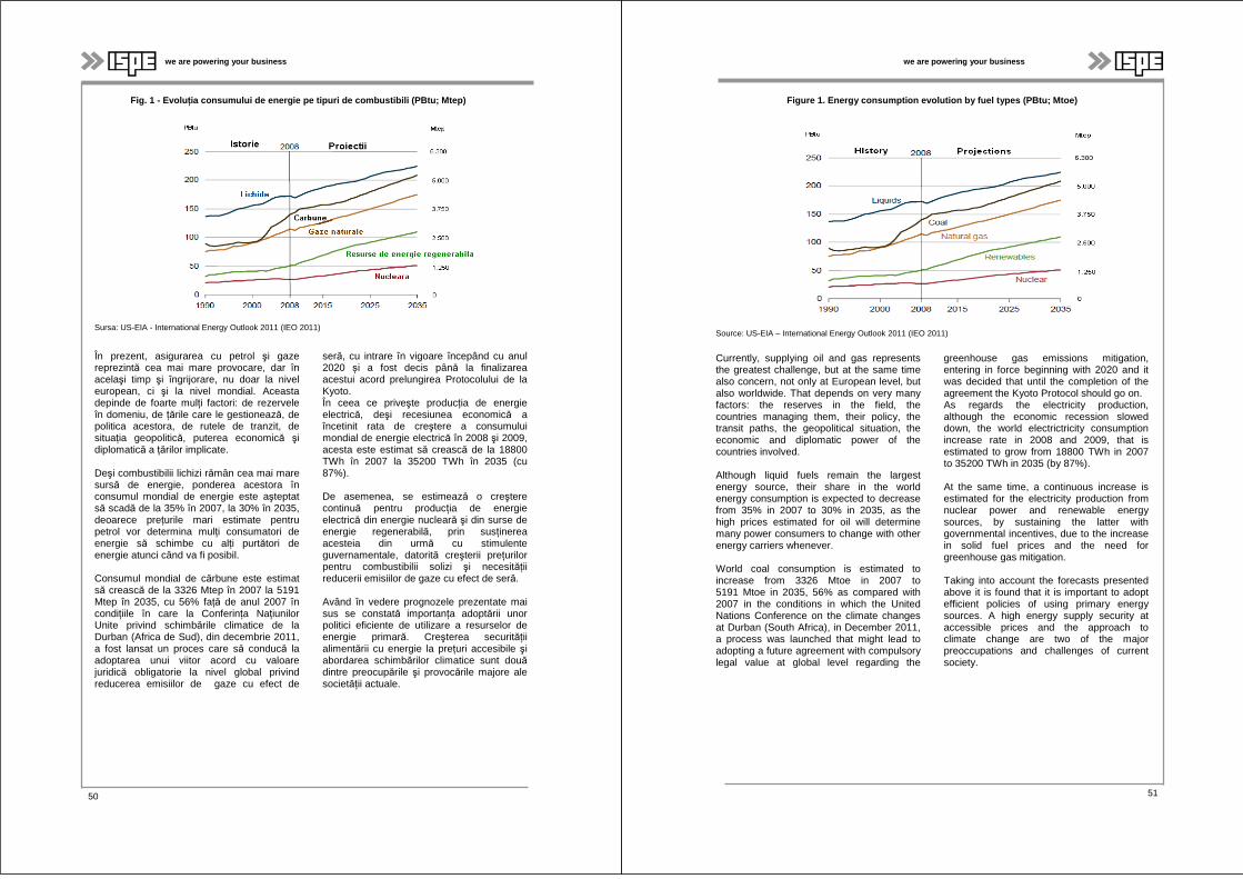
we are powering your business
Fig. 1 - Evolu ţia consumului de energie pe tipuri de combustibili (PBtu; Mtep)
Sursa: US-EIA - International Energy Outlook 2011 (IEO 2011)
În prezent, asigurarea cu petrol şi gaze reprezintă cea mai mare provocare, dar în acelaşi timp şi îngrijorare, nu doar la nivel european, ci şi la nivel mondial. Aceasta depinde de foarte mulţi factori: de rezervele în domeniu, de ţările care le gestionează, de politica acestora, de rutele de tranzit, de situaţia geopolitică, puterea economică şi diplomatică a ţărilor implicate.
Deşi combustibilii lichizi rămân cea mai mare sursă de energie, ponderea acestora în consumul mondial de energie este aşteptat să scadă de la 35% în 2007, la 30% în 2035, deoarece preţurile mari estimate pentru petrol vor determina mulţi consumatori de energie să schimbe cu alţi purtători de energie atunci când va fi posibil.
Consumul mondial de cărbune este estimat să crească de la 3326 Mtep în 2007 la 5191 Mtep în 2035, cu 56% faţă de anul 2007 în condițiile în care la Conferința Națiunilor Unite privind schimbările climatice de la Durban (Africa de Sud), din decembrie 2011, a fost lansat un proces care să conducă la adoptarea unui viitor acord cu valoare juridică obligatorie la nivel global privind reducerea emisiilor de gaze cu efect de
seră, cu intrare în vigoare începând cu anul 2020 și a fost decis până la finalizarea acestui acord prelungirea Protocolului de la Kyoto. În ceea ce priveşte producţia de energie electrică, deşi recesiunea economică a încetinit rata de creştere a consumului mondial de energie electrică în 2008 şi 2009, acesta este estimat să crească de la 18800 TWh în 2007 la 35200 TWh în 2035 (cu 87%).
De asemenea, se estimează o creştere continuă pentru producţia de energie electrică din energie nucleară şi din surse de energie regenerabilă, prin susţinerea acesteia din urmă cu stimulente guvernamentale, datorită creşterii preţurilor pentru combustibilii solizi şi necesităţii reducerii emisiilor de gaze cu efect de seră.
Având în vedere prognozele prezentate mai sus se constată importanța adoptării unor politici eficiente de utilizare a resurselor de energie primară. Creşterea securităţii alimentării cu energie la preţuri accesibile şi abordarea schimbărilor climatice sunt douădintre preocupările şi provocările majore ale societăţii actuale.
50
we are powering your business
Figure 1. Energy consumption evolution by fuel types (PBtu; Mtoe)
Source: US-EIA – International Energy Outlook 2011 (IEO 2011)
Currently, supplying oil and gas represents the greatest challenge, but at the same time also concern, not only at European level, but also worldwide. That depends on very many factors: the reserves in the field, the countries managing them, their policy, the transit paths, the geopolitical situation, the economic and diplomatic power of the countries involved.
Although liquid fuels remain the largest energy source, their share in the world energy consumption is expected to decrease from 35% in 2007 to 30% in 2035, as the high prices estimated for oil will determine many power consumers to change with other energy carriers whenever.
World coal consumption is estimated to increase from 3326 Mtoe in 2007 to 5191 Mtoe in 2035, 56% as compared with 2007 in the conditions in which the United Nations Conference on the climate changes at Durban (South Africa), in December 2011, a process was launched that might lead to adopting a future agreement with compulsory legal value at global level regarding the
greenhouse gas emissions mitigation, entering in force beginning with 2020 and it was decided that until the completion of the agreement the Kyoto Protocol should go on. As regards the electricity production, although the economic recession slowed down, the world electrictricity consumption increase rate in 2008 and 2009, that is estimated to grow from 18800 TWh in 2007 to 35200 TWh in 2035 (by 87%).
At the same time, a continuous increase is estimated for the electricity production from nuclear power and renewable energy sources, by sustaining the latter with governmental incentives, due to the increase in solid fuel prices and the need for greenhouse gas mitigation.
Taking into account the forecasts presented above it is found that it is important to adopt efficient policies of using primary energy sources. A high energy supply security at accessible prices and the approach to climate change are two of the major preoccupations and challenges of current society.
51
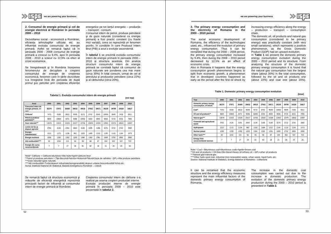
we are powering your business
2. Consumul de energie primar ă şi cel de energie electric ă al României în perioada 2000 – 2010
Dezvoltarea social - economică a României, eficiența tehnologiilor utilizate etc. au influențat evoluția consumului de energie primară. Astfel se remarcă faptul că în perioada 2000 - 2008 consumul de energie primară a crescut cu 9,4%, apoi în perioada 2008 - 2010 a scăzut cu 12,5% ca efect al crizei economice.
Se înregistrează şi în România începerea fenomenului de decuplare a creşterii consumului de energie de creşterea economică, fenomen care în ţările dezvoltate s-a înregistrat încă din perioada de dupăprimul şoc petrolier prin creşterea eficienţei
energetice pe tot lanţul energetic – producţie – transport - consum. Consumul intern de petrol, produse petroliere şi de gaze naturale (considerat ca energie primară) a fost practic constant (cu foarte mici variaţii), ceea ce reprezintă un fenomen pozitiv, în condiţiile în care Produsul Intern Brut (PIB) a avut o evoluţie ascendentă.
În tabelul 1 se prezintă evoluția consumului intern de energie primară în perioada 2000 – 2010 și structura acestuia. Din analiza structurii consumului intern de energie primară se constată faptul că consumul de gaze naturale are ponderea cea mai mare (circa 30%) în total consum, urmat de cel al petrolului și produselor petroliere (circa 22%) și al cărbunelui (circa 20%).
Tabelul 1. Evolu ţia consumului intern de energie primar ă [mii tep]
Notă:* Cărbune = Cărbune bituminos+Alte huile+lignit+cărbune brun **Petrol şi produse petroliere = Ţiţei-Benzină-Petroluri-Motorină-Păcură-Gaze de rafinărie - GPL+Alte produse petroliere ***Gaze naturale=gaze naturale. ****Alți combustibili=Turbă,deșeuri industriale(neregenerabile),deșeuri urbane,biocombustibili lichizi,etc. Sursa: Institutul Naţional de Statistică, Balanţa Energetică a României – colecţii
Se remarcă faptul că structura economică şi măsurile de eficienţă energetică reprezintăprincipalii factori de influenţă ai consumului intern de energie primară al României.
Creşterea consumului intern de cărbune s-a realizat pe seama creşterii producţiei interne. Evoluţia producţiei interne de energie primară în perioada 2000 – 2010 este prezentată în tabelul 2.
Anul 2000 2001 2002 2003 2004 2005 2006 2007 2008 2009 2010
Consumul intern de energie primar ă, din care:
36374 37971 36480 39032 39018 37932 39571 39159 39799 34328 34817
Cărbune* 7475 8169 8812 9509 9172 8742 9540 10064 9649 7436 6911
Petrol şi produse petroliere** 9808 10804 9371 9088 10092 9163 9840 9658 9719 8331 7855
Gaze naturale*** 13679 13315 13326 15317 13766 13820 14308 12862 12476 10642 10897
Lemne de foc şi deşeuri agricole 2763 2134 2351 2844 3134 3185 3185 3275 3710 3742 3982
Energie hidroelectric ă 1212 1172 1136 962 1320 1489 1212 1195 1115 1164 1573
Energie nuclear ă 1338 1335 1352 1203 1360 1362 1381 1890 2752 2881 2850
Al ţi combustibili**** 92 1034 115 93 93 88 87 194 352 107 723
Energie din surse neconven ţionale 7 7 17 18 81 82 18 21 26 25 26
52
we are powering your business
2. The primary energy consumption and the electricity of Romania in the 2000 – 2010 period
The social economic development of Romania, the efficiency of the technologies used, etc., influenced the evolution of primary energy consumption. Thus it can be remarked that during the 2000 – 2008 period, the primary energy consumption increased by 9.4%, then during the 2008 – 2010 period decreased by 12.5% as an effect of economic crisis. Also in Romania it happens that the energy consumption growth phenomenon begins to split from economic growth, a phenomenon that in developed countries happened as early as the period after the first oil shock by
increasing energy efficiency along the energy – production – transport – consumption chain. The domestic oil, oil products and natural gas consumption (considered to be primary energy) was practically constant (with very small variations), which represents a positive phenomenon, as the Gross Domestic Product (GDP) had an upward evolution. In Table 1 we present the domestic primary energy consumption evolution during the 2000 – 2010 period and its structure. From analyzing the structure of the domestic primary energy consumption it is found that the natural gas consumption has the largest share (about 30%) in the total consumption, followed by the oil and oil products one (about 22%) and coal one (about 20%).
Table 1. Domestic primary energy consumption evolut ion [ktoe]
Note:* Coal = Bituminous coal+bituminous coals+lignite+brown coal **Oil and oil products = Oil-Gas-Oils-Diesel-Heavy oil-refinery oil – GPL+other oil products ***Natural gas=natural gas ****Other fuels=peat coal, industrial (non-renewable) waste, urban waste, liquid fuels, etc. Source: National Institute of Statistics, Energy Balance of Romania – collections
It can be remarked that the economic structure and the energy efficiency measures represent the main influential factors of the domestic primary energy consumption of Romania.
The increase in the domestic coal consumption was carried out due to the increase in domestic production. The evolution of the domestic primary energy production during the 2000 – 2010 period is presented in Table 2.
Year 2000 2001 2002 2003 2004 2005 2006 2007 2008 2009 2010
Domestic primary energy consumption, of which: 36374 37971 36480 39032 39018 37932 39571 39159 39799 34328 34817
Coal* 7475 8169 8812 9509 9172 8742 9540 10064 9649 7436 6911
Oil and oil products** 9808 10804 9371 9088 10092 9163 9840 9658 9719 8331 7855
Natural gas*** 13679 13315 13326 15317 13766 13820 14308 12862 12476 10642 10897
Firewood and agricultural waste 2763 2134 2351 2844 3134 3185 3185 3275 3710 3742 3982
Hydropower 1212 1172 1136 962 1320 1489 1212 1195 1115 1164 1573
Nuclear power 1338 1335 1352 1203 1360 1362 1381 1890 2752 2881 2850
Other fuels**** 92 1034 115 93 93 88 87 194 352 107 723
Energy from unconventional sources 7 7 17 18 81 82 18 21 26 25 26
53
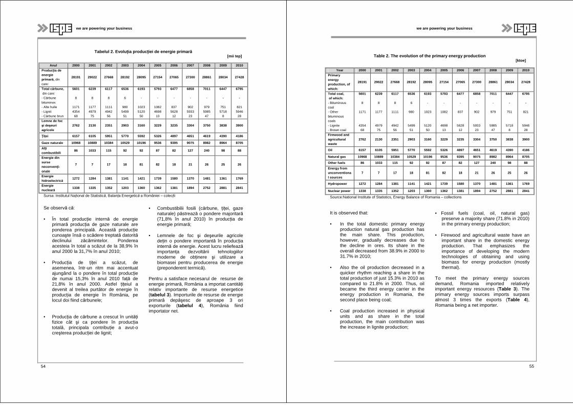
we are powering your business
Tabelul 2. Evolu ţia produc ţiei de energie primar ă[mii tep]
Anul 2000 2001 2002 2003 2004 2005 2006 2007 2008 2009 2010
Produc ţia de energie primar ă, din care:
28191 29022 27668 28192 28095 27154 27065 27300 28861 28034 27428
Total c ărbune, din care:- Cărbune bituminos - Alte huile - Lignit - Cărbune brun
5601
8
1171 4354
68
6239
8
1177 4979 75
6117
8
1111 4942 56
6536
6
980 5499 51
6193
-
1023 5120 50
5793
-
1082 4698 13
6477
-
837 5628 12
6858
-
902 5933 23
7011
-
979 5985 47
6447
-
751 5718
8
6795
-
821 5946 28
Lemne de foc şi deşeuri agricole
2762 2130 2351 2903 3160 3229 3235 3304 3750 3838 3900
Ţiţei 6157 6105 5951 5770 5592 5326 4897 4651 4619 4390 4186
Gaze naturale 10968 10889 10384 10529 10196 9536 93 95 9075 8982 8964 8705
Al ţi combustibili
86 1033 115 92 92 87 82 127 240 98 88
Energie din surse neconven ţi-onale
7 7 17 18 81 82 18 21 26 25 26
Energie hidroelectric ă
1272 1284 1381 1141 1421 1739 1580 1370 1481 1361 1769
Energie nuclear ă
1338 1335 1352 1203 1360 1362 1381 1894 2752 2881 2841
Sursa: Institutul Naţional de Statistică, Balanţa Energetică a României – colecţii
Se observă că:
• În total producţie internă de energie primară producția de gaze naturale are ponderea principală. Această producţie cunoaşte însă o scădere treptată datoritădeclinului zăcămintelor. Ponderea acesteia în total a scăzut de la 38,9% în anul 2000 la 31,7% în anul 2010;
• Producţia de ţiţei a scăzut, de asemenea, într-un ritm mai accentuat ajungând la o pondere în total producție de numai 15,3% în anul 2010 faţă de 21,8% în anul 2000. Astfel ţiţeiul a devenit al treilea purtător de energie în producţia de energie în România, pe locul doi fiind cărbunele;
• Producţia de cărbune a crescut în unităţi fizice cât şi ca pondere în producţia totală, principala contribuţie a avut-o creşterea producţiei de lignit;
• Combustibilii fosili (cărbune, ţiţei, gaze naturale) păstrează o pondere majoritară(71,8% în anul 2010) în producţia de energie primară;
• Lemnele de foc şi deşeurile agricole deţin o pondere importantă în producţia internă de energie. Acest lucru reliefeazăimportanţa dezvoltării tehnologiilor moderne de obţinere şi utilizare a biomasei pentru producerea de energie (preponderent termică).
Pentru a satisface necesarul de resurse de energie primară, România a importat cantităţi relativ importante de resurse energetice (tabelul 3 ). Importurile de resurse de energie primară depăşesc de aproape 3 ori exporturile (tabelul 4 ), România fiind importator net.
54
we are powering your business
Table 2. The evolution of the primary energy produc tion [ktoe]
Year 2000 2001 2002 2003 2004 2005 2006 2007 2008 2009 2010
Primary energy production, of which:
28191 29022 27668 28192 28095 27154 27065 27300 28861 28034 27428
Total coal, of which: - Bituminous coal - Other bituminous coals - Lignite - Brown coal
5601
8
1171
4354 68
6239
8
1177
4979 75
6117
8
1111
4942 56
6536
6
980
5499 51
6193
-
1023
5120 50
5793
-
1082
4698 13
6477
-
837
5628 12
6858
-
902
5933 23
7011
-
979
5985 47
6447
-
751
5718 8
6795
-
821
5946 28
Firewood and agricultural waste
2762 2130 2351 2903 3160 3229 3235 3304 3750 3838 3900
Oil 6157 6105 5951 5770 5592 5326 4897 4651 4619 4390 4186
Natural gas 10968 10889 10384 10529 10196 9536 9395 9075 8982 8964 8705
Other fuels 86 1033 115 92 92 87 82 127 240 98 88
Energy from unconventional sources
7 7 17 18 81 82 18 21 26 25 26
Hydropower 1272 1284 1381 1141 1421 1739 1580 1370 1481 1361 1769
Nuclear power 1338 1335 1352 1203 1360 1362 1381 18 94 2752 2881 2841
Source:National Institute of Statistics, Energy Balance of Romania – collections
It is observed that:
• In the total domestic primary energy production natural gas production has the main share. This production, however, gradually decreases due to the decline in ores. Its share in the overall decreased from 38.9% in 2000 to 31.7% in 2010;
• Also the oil production decreased in a quicker rhythm reaching a share in the total production of just 15.3% in 2010 as compared to 21.8% in 2000. Thus, oil became the third energy carrier in the energy production in Romania, the second place being coal;
• Coal production increased in physical units and as share in the total production, the main contribution was the increase in lignite production;
• Fossil fuels (coal, oil, natural gas) preserve a majority share (71.8% in 2010) in the primary energy production;
• Firewood and agricultural waste have an important share in the domestic energy production. That emphasizes the importance of developing the modern technologies of obtaining and using biomass for energy production (mostly thermal).
To meet the primary energy sources demand, Romania imported relatively important energy resources (Table 3 ). The primary energy sources imports surpass almost 3 times the exports (Table 4 ), Romania being a net importer.
55
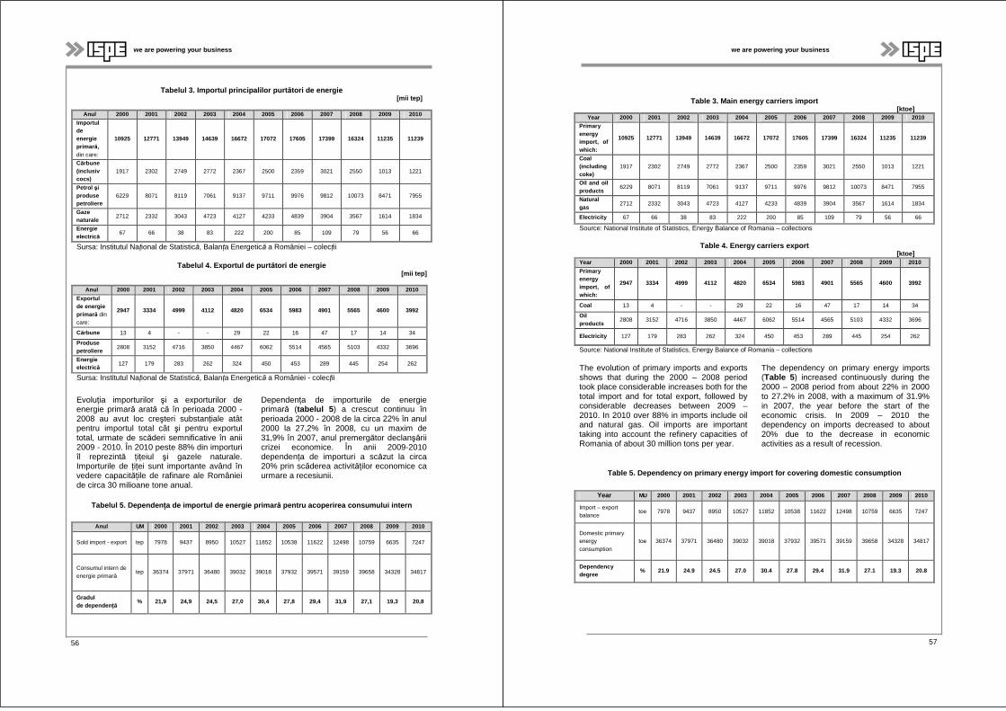
we are powering your business
Tabelul 3. Importul principalilor purt ători de energie [mii tep]
Anul 2000 2001 2002 2003 2004 2005 2006 2007 2008 2009 2010
Importul de energie primar ă, din care:
10925 12771 13949 14639 16672 17072 17605 17399 16324 11235 11239
Cărbune (inclusiv cocs)
1917 2302 2749 2772 2367 2500 2359 3021 2550 1013 1221
Petrol şi produse petroliere
6229 8071 8119 7061 9137 9711 9976 9812 10073 8471 7955
Gaze naturale
2712 2332 3043 4723 4127 4233 4839 3904 3567 1614 1834
Energie electric ă
67 66 38 83 222 200 85 109 79 56 66
Sursa: Institutul Naţional de Statistică, Balanţa Energetică a României – colecţii
Tabelul 4. Exportul de purt ători de energie [mii tep]
Anul 2000 2001 2002 2003 2004 2005 2006 2007 2008 2009 2010
Exportul de energie primar ă din care:
2947 3334 4999 4112 4820 6534 5983 4901 5565 4600 3992
Cărbune 13 4 - - 29 22 16 47 17 14 34
Produse petroliere
2808 3152 4716 3850 4467 6062 5514 4565 5103 4332 3696
Energie electric ă
127 179 283 262 324 450 453 289 445 254 262
Sursa: Institutul Naţional de Statistică, Balanţa Energetică a României - colecţii
Evoluţia importurilor şi a exporturilor de energie primară arată că în perioada 2000 - 2008 au avut loc creşteri substanţiale atât pentru importul total cât şi pentru exportul total, urmate de scăderi semnificative în anii 2009 - 2010. În 2010 peste 88% din importuri îl reprezintă ţiţeiul şi gazele naturale. Importurile de țiței sunt importante având în vedere capacitățile de rafinare ale României de circa 30 milioane tone anual.
Dependenţa de importurile de energie primară (tabelul 5 ) a crescut continuu în perioada 2000 - 2008 de la circa 22% în anul 2000 la 27,2% în 2008, cu un maxim de 31,9% în 2007, anul premergător declanşării crizei economice. În anii 2009-2010 dependenţa de importuri a scăzut la circa 20% prin scăderea activităţilor economice ca urmare a recesiunii.
Tabelul 5. Dependen ţa de importul de energie primar ă pentru acoperirea consumului intern
Anul UM 2000 2001 2002 2003 2004 2005 2006 2007 2008 2009 2010
Sold import - export tep 7978 9437 8950 10527 11852 10538 11622 12498 10759 6635 7247
Consumul intern de energie primară
tep 36374 37971 36480 39032 39018 37932 39571 39159 39658 34328 34817
Gradul de dependen ţă
% 21,9 24,9 24,5 27,0 30,4 27,8 29,4 31,9 27,1 19,3 20,8
54 56
we are powering your business
Table 3. Main energy carriers import [ktoe]
Year 2000 2001 2002 2003 2004 2005 2006 2007 2008 2009 2010 Primary energy import, of which:
10925 12771 13949 14639 16672 17072 17605 17399 16324 11235 11239
Coal (including coke)
1917 2302 2749 2772 2367 2500 2359 3021 2550 1013 1221
Oil and oil products
6229 8071 8119 7061 9137 9711 9976 9812 10073 8471 7955
Natural gas
2712 2332 3043 4723 4127 4233 4839 3904 3567 1614 1834
Electricity 67 66 38 83 222 200 85 109 79 56 66
Source: National Institute of Statistics, Energy Balance of Romania – collections
Table 4. Energy carriers export [ktoe]
Year 2000 2001 2002 2003 2004 2005 2006 2007 2008 2009 2010
Primary energy import, of which:
2947 3334 4999 4112 4820 6534 5983 4901 5565 4600 3992
Coal 13 4 - - 29 22 16 47 17 14 34
Oil products
2808 3152 4716 3850 4467 6062 5514 4565 5103 4332 3696
Electricity 127 179 283 262 324 450 453 289 445 254 262
Source: National Institute of Statistics, Energy Balance of Romania – collections
The evolution of primary imports and exports shows that during the 2000 – 2008 period took place considerable increases both for the total import and for total export, followed by considerable decreases between 2009 – 2010. In 2010 over 88% in imports include oil and natural gas. Oil imports are important taking into account the refinery capacities of Romania of about 30 million tons per year.
The dependency on primary energy imports (Table 5 ) increased continuously during the 2000 – 2008 period from about 22% in 2000 to 27.2% in 2008, with a maximum of 31.9% in 2007, the year before the start of the economic crisis. In 2009 – 2010 the dependency on imports decreased to about 20% due to the decrease in economic activities as a result of recession.
Table 5. Dependency on primary energy import for co vering domestic consumption
Year MU 2000 2001 2002 2003 2004 2005 2006 2007 2008 2009 2010
Import – export balance
toe 7978 9437 8950 10527 11852 10538 11622 12498 10759 6635 7247
Domestic primary energy consumption
toe 36374 37971 36480 39032 39018 37932 39571 39159 39658 34328 34817
Dependency degree
% 21.9 24.9 24.5 27.0 30.4 27.8 29.4 31.9 27.1 19.3 20.8
57
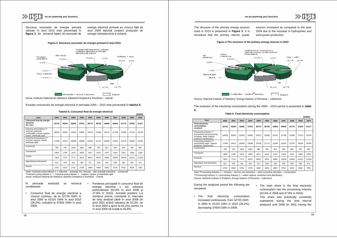
we are powering your business
Structura resurselor de energie primarăutilizate în anul 2010 este prezentată în figura 2 . Se remarcă faptul că resursele de
energie electrică primară au crescut față de anul 2009 datorită creșterii producției de energie hidroelectrică și eoliană.
Figura 2. Structura resurselor de energie primar ă în anul 2010
Sursa: Institutul Naţional de Statistică, Balanţa Energetică a României – colecţii
Evoluţia consumului de energie electrică în perioada 2000 – 2010 este prezentată în tabelul 6 .
Tabelul 6. Consumul final de energie electric ă[GWh]
Anul 2000 2001 2002 2003 2004 2005 2006 2007 2008 2009 2010
Consumul final de energie electric ă, din care:
32735 36294 35569 37501 38774 38756 40965 40949 41775 37605 41317
Industria prelucrătoare 1* (exclusiv prelucrări combustibil, inclusiv captare, tratare, distribuţie apă)
18529 19361 21062 20681 24073 22460 23121 21758 21993 17214 19734
Industria prelucrătoare 2** (exclusiv captare, tratare, distribuţie apă)
17386 18411 20096 19856 23235 21712 22394 21032 21370 16620 18790
Construcţii 755 745 1029 1062 680 703 813 934 842 793 697
Transporturi 1859 1785 1970 1829 1617 1610 1347 1463 1401 1383 1355
Casnic 7652 7724 7771 8243 8043 9234 9999 10039 10040 11021 11329
Agricultură şi silvicultură611 479 421 343 271 228 442 539 555 493 671
Servicii 2702 5552 2701 4749 3586 4000 4900 5720 6432 6526 7581
Notă: *Industrie prelucrătoare 1 = Industrie – extracţia min. feroase – alte activităţi extractive – construcţii **Industrie prelucrătoare 2 = Industrie prelucrătoare 1 – captare, tartare şi distribuţie apăSursa: Institutul Naţional de Statistică, Balanţa Energetică a României – colecţii
În perioada analizată se remarcăurmătoarele:
• Consumul final de energie electrică a crescut continuu, de la 32735 GWh în anul 2000 la 41315 GWh în anul 2010 (26,2%), scăzând la 37605 GWh în anul 2009;
• Ponderea principală în consumul final de energie electrică o are industria prelucrătoare (52,6% în anul 2008 şi 47,8% în 2010). Această pondere s-a menţinut practic constantă în intervalul de timp analizat până în anul 2008 (în anul 2001 având valoarea de 53,3%, iar în anul 2004 a ajuns la 62,1%), pentru ca în anul 2009 să scadă la 45,8%;
58
we are powering your business
The structure of the primary energy sources used in 2010 is presented in Figure 2 . It is remarked that the primary electric power
sources increased as compared to the year 2009 due to the increase in hydropower and wind power production.
Figure 2.The structure of the primary energy source s in 2010
Source: National Institute of Statistics, Energy balance of Romania – collections
The evolution of the electricity consumption during the 2000 – 2010 period is presented in table 6. Table 6. Final electricity consumption
[GWh]Year 2000 2001 2002 2003 2004 2005 2006 2007 2008 2009 2010
Final electricity consumption, of which:
32735 36294 35569 37501 38774 38756 40965 40949 41775 37605 41317
Processing industry 1* (exclusively fuel processing, including water capture, treatment, distribution)
18529 19361 21062 20681 24073 22460 23121 21758 21993 17214 19734
Processing industry 2** (exclusively water capture, treatment, distribution)
17386 18411 20096 19856 23235 21712 22394 21032 21370 16620 18790
Construction 755 745 1029 1062 680 703 813 934 842 793 697
Transports 1859 1785 1970 1829 1617 1610 1347 1463 1401 1383 1355
Domestic 7652 7724 7771 8243 8043 9234 9999 10039 10040 11021 11329
Agriculture and silviculture 611 479 421 343 271 228 442 539 555 493 671
Services 2702 5552 2701 4749 3586 4000 4900 5720 6432 6526 7581
Note:*Processing industry 1 = Industry – ferrous ore extraction – other extractive activities – construction **Processing industry 2 = processing industry 1 – water capture, treatment and distribution Source: National Institute of Statistics, Energy balance of Romania – collections
During the analyzed period the following are remarked:
• The final electricity consumption increased continuously, from 32735 GWh in 2000 to 41315 GWh in 2010 (26.2%), decreasing 37605 GWh in 2009;
• The main share in the final electricity consumption has the processing industry (52.6% in 2008 and 47.8% in 2010). This share was practically constantly maintaneid during the time interval analyzed until 2008 (in 2001 having the
59
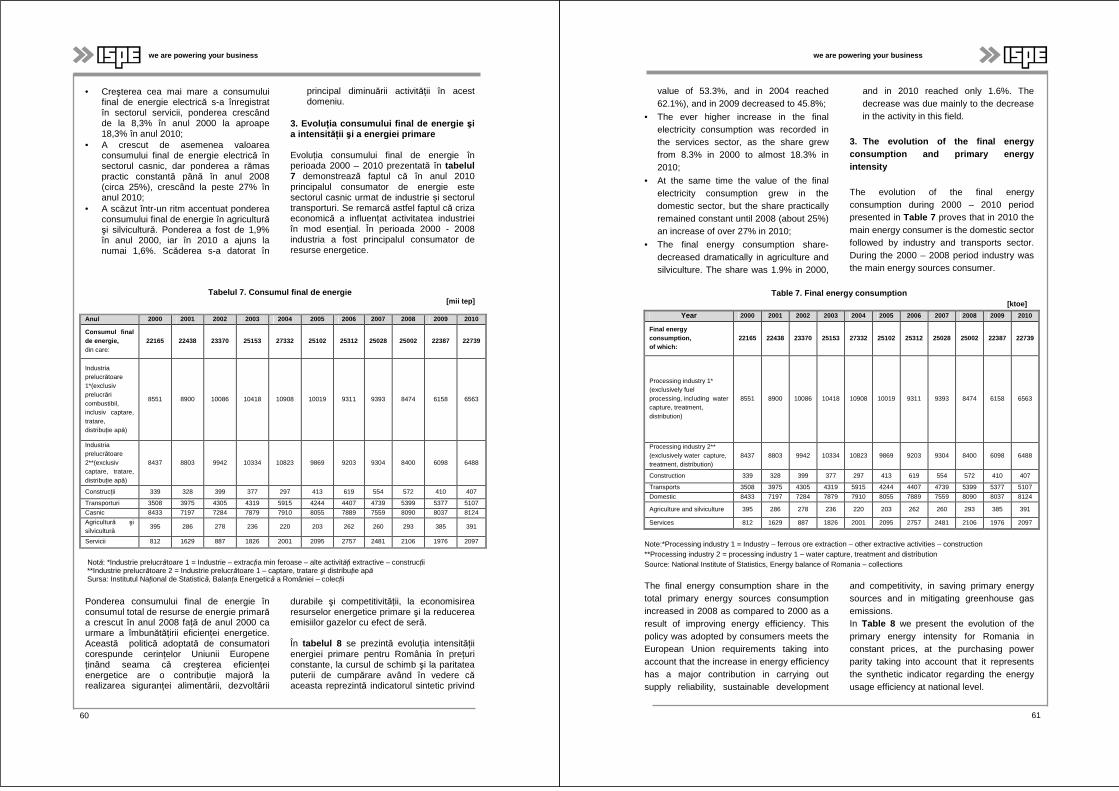
we are powering your business
• Creşterea cea mai mare a consumului final de energie electrică s-a înregistrat în sectorul servicii, ponderea crescând de la 8,3% în anul 2000 la aproape 18,3% în anul 2010;
• A crescut de asemenea valoarea consumului final de energie electrică în sectorul casnic, dar ponderea a rămas practic constantă până în anul 2008 (circa 25%), crescând la peste 27% în anul 2010;
• A scăzut într-un ritm accentuat ponderea consumului final de energie în agriculturăşi silvicultură. Ponderea a fost de 1,9% în anul 2000, iar în 2010 a ajuns la numai 1,6%. Scăderea s-a datorat în
principal diminuării activităţii în acest domeniu.
3. Evolu ţia consumului final de energie şi a intensit ăţii şi a energiei primare
Evoluţia consumului final de energie în perioada 2000 – 2010 prezentată în tabelul 7 demonstrează faptul că în anul 2010 principalul consumator de energie este sectorul casnic urmat de industrie și sectorul transporturi. Se remarcă astfel faptul că criza economică a influențat activitatea industriei în mod esențial. În perioada 2000 - 2008 industria a fost principalul consumator de resurse energetice.
Tabelul 7. Consumul final de energie [mii tep]
Anul 2000 2001 2002 2003 2004 2005 2006 2007 2008 2009 2010
Consumul final de energie, din care:
22165 22438 23370 25153 27332 25102 25312 25028 25002 22387 22739
Industria prelucrătoare 1*(exclusiv prelucrări combustibil, inclusiv captare, tratare, distribuţie apă)
8551 8900 10086 10418 10908 10019 9311 9393 8474 6158 6563
Industria prelucrătoare 2**(exclusiv captare, tratare, distribuţie apă)
8437 8803 9942 10334 10823 9869 9203 9304 8400 6098 6488
Construcţii 339 328 399 377 297 413 619 554 572 410 407
Transporturi 3508 3975 4305 4319 5915 4244 4407 4739 5399 5377 5107
Casnic 8433 7197 7284 7879 7910 8055 7889 7559 8090 8037 8124
Agricultură şi silvicultură
395 286 278 236 220 203 262 260 293 385 391
Servicii 812 1629 887 1826 2001 2095 2757 2481 2106 1976 2097
Notă: *Industrie prelucrătoare 1 = Industrie – extracţia min feroase – alte activităţi extractive – construcţii
**Industrie prelucrătoare 2 = Industrie prelucrătoare 1 – captare, tratare şi distribuţie apă Sursa: Institutul Naţional de Statistică, Balanţa Energetică a României – colecţii Ponderea consumului final de energie în consumul total de resurse de energie primarăa crescut în anul 2008 faţă de anul 2000 ca urmare a îmbunătăţirii eficienţei energetice. Această politică adoptată de consumatori corespunde cerințelor Uniunii Europene ținând seama că creşterea eficienţei energetice are o contribuţie majoră la realizarea siguranţei alimentării, dezvoltării
durabile şi competitivităţii, la economisirea resurselor energetice primare şi la reducerea emisiilor gazelor cu efect de seră.
În tabelul 8 se prezintă evoluţia intensităţii energiei primare pentru România în preţuri constante, la cursul de schimb şi la paritatea puterii de cumpărare având în vedere căaceasta reprezintă indicatorul sintetic privind
60
we are powering your business
value of 53.3%, and in 2004 reached 62.1%), and in 2009 decreased to 45.8%;
• The ever higher increase in the final electricity consumption was recorded in the services sector, as the share grew from 8.3% in 2000 to almost 18.3% in 2010;
• At the same time the value of the final electricity consumption grew in the domestic sector, but the share practically remained constant until 2008 (about 25%) an increase of over 27% in 2010;
• The final energy consumption share- decreased dramatically in agriculture and silviculture. The share was 1.9% in 2000,
and in 2010 reached only 1.6%. The decrease was due mainly to the decrease in the activity in this field.
3. The evolution of the final energy consumption and primary energy intensity
The evolution of the final energy consumption during 2000 – 2010 period presented in Table 7 proves that in 2010 the main energy consumer is the domestic sector followed by industry and transports sector. During the 2000 – 2008 period industry was the main energy sources consumer.
Table 7. Final energy consumption [ktoe]
Year 2000 2001 2002 2003 2004 2005 2006 2007 2008 2009 2010
Final energy consumption, of which:
22165 22438 23370 25153 27332 25102 25312 25028 25002 22387 22739
Processing industry 1* (exclusively fuel processing, including water capture, treatment, distribution)
8551 8900 10086 10418 10908 10019 9311 9393 8474 6158 6563
Processing industry 2** (exclusively water capture, treatment, distribution)
8437 8803 9942 10334 10823 9869 9203 9304 8400 6098 6488
Construction 339 328 399 377 297 413 619 554 572 410 407
Transports 3508 3975 4305 4319 5915 4244 4407 4739 5399 5377 5107
Domestic 8433 7197 7284 7879 7910 8055 7889 7559 8090 8037 8124
Agriculture and silviculture 395 286 278 236 220 203 262 260 293 385 391
Services 812 1629 887 1826 2001 2095 2757 2481 2106 1976 2097
Note:*Processing industry 1 = Industry – ferrous ore extraction – other extractive activities – construction **Processing industry 2 = processing industry 1 – water capture, treatment and distribution Source: National Institute of Statistics, Energy balance of Romania – collections
The final energy consumption share in the total primary energy sources consumption increased in 2008 as compared to 2000 as a result of improving energy efficiency. This policy was adopted by consumers meets the European Union requirements taking into account that the increase in energy efficiency has a major contribution in carrying out supply reliability, sustainable development
and competitivity, in saving primary energy sources and in mitigating greenhouse gas emissions. In Table 8 we present the evolution of the primary energy intensity for Romania in constant prices, at the purchasing power parity taking into account that it represents the synthetic indicator regarding the energy usage efficiency at national level.
61
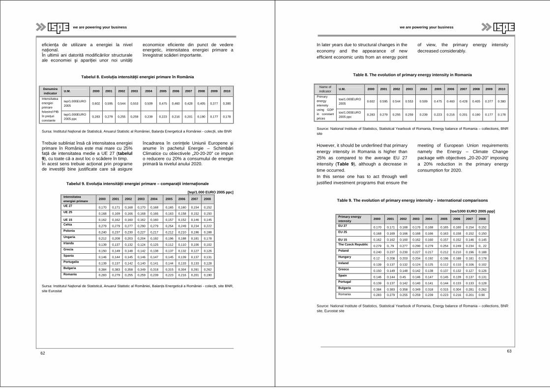
we are powering your business
eficiența de utilizare a energiei la nivel național. În ultimii ani datorită modificărilor structurale ale economiei şi apariţiei unor noi unităţi
economice eficiente din punct de vedere energetic, intensitatea energiei primare a înregistrat scăderi importante.
Tabelul 8. Evolu ţia intensit ăţii energiei primare în România
Denumire indicator
U.M. 2000 2001 2002 2003 2004 2005 2006 2007 2008 2009 2010
Intensitatea energiei primare folosind PIB în preţuri constante
tep/1.000EURO 2005
0,602 0,595 0,544 0,553 0,509 0,475 0,460 0,428 0,405 0,377 0,380
tep/1.000EURO 2005 ppc
0,283 0,279 0,255 0,259 0,239 0,223 0,216 0,201 0,190 0,177 0,178
Sursa: Institutul Naţional de Statistică, Anuarul Statistic al României, Balanţa Energetică a României - colecţii, site BNR
Trebuie subliniat însă că intensitatea energiei primare în România este mai mare cu 25% faţă de intensitatea medie a UE 27 (tabelul 9), cu toate că a avut loc o scădere în timp. În acest sens trebuie acționat prin programe de investiții bine justificate care să asigure
încadrarea în cerințele Uniunii Europene și anume în pachetul Energie – Schimbări Climatice cu obiectivele „20-20-20” ce impun o reducere cu 20% a consumului de energie primară la nivelul anului 2020.
Tabelul 9. Evolu ţia intensit ăţii energiei primare – compara ţii interna ţionale
[tep/1.000 EURO 2005 ppc] Intensitatea energiei primare
2000 2001 2002 2003 2004 2005 2006 2007 2008
UE 27 0,170 0,171 0,168 0,170 0,168 0,165 0,160 0,154 0,152
UE 25 0,168 0,169 0,166 0,168 0,166 0,163 0,158 0,152 0,150
UE 15 0,162 0,162 0,160 0,162 0,160 0,157 0,152 0,146 0,145
Cehia 0,279 0,279 0,277 0,290 0,279 0,254 0,249 0,234 0,222
Polonia 0,240 0,237 0,230 0,227 0,217 0,212 0,210 0,196 0,188
Ungaria 0,212 0,208 0,203 0,204 0,192 0,196 0,188 0,181 0,178
Irlanda 0,139 0,137 0,132 0,124 0,125 0,112 0,110 0,106 0,102
Grecia 0,150 0,149 0,148 0,142 0,138 0,137 0,132 0,127 0,126
Spania 0,146 0,144 0,145 0,146 0,147 0,145 0,139 0,137 0,131
Portugalia 0,139 0,137 0,142 0,140 0,141 0,144 0,133 0,133 0,128
Bulgaria 0,384 0,383 0,358 0,349 0,318 0,315 0,304 0,281 0,262
Romania 0,283 0,279 0,255 0,259 0,239 0,223 0,216 0,201 0,190
Sursa: Institutul Naţional de Statistică, Anuarul Statistic al României, Balanţa Energetică a României - colecţii, site BNR, site Eurostat
64 62
we are powering your business
In later years due to structural changes in the economy and the appearance of new efficient economic units from an energy point
of view, the primary energy intensity decreased considerably.
Table 8. The evolution of primary energy intensity in Romania
Name of indicator
U.M. 2000 2001 2002 2003 2004 2005 2006 2007 2008 2009 2010
Primary energy intensity using GDP in constant prices
toe/1.000EURO 2005
0.602 0.595 0.544 0.553 0.509 0.475 0.460 0.428 0.405 0.377 0.380
toe/1.000EURO 2005 ppc
0.283 0.279 0.255 0.259 0.239 0.223 0.216 0.201 0.190 0.177 0.178
Source: National Institute of Statistics, Statistical Yearbook of Romania, Energy balance of Romania – collections, BNR site
However, it should be underlined that primary energy intensity in Romania is higher than 25% as compared to the average EU 27 intensity (Table 9 ), although a decrease in time occurred. In this sense one has to act through well justified investment programs that ensure the
meeting of European Union requirements namely the Energy – Climate Change package with objectives „20-20-20” imposing a 20% reduction in the primary energy consumption for 2020.
Table 9. The evolution of primary energy intensity – international comparisons
[toe/1000 EURO 2005 ppp]Primary energy intensity
2000 2001 2002 2003 2004 2005 2006 2007 2008
EU 27 0.170 0.171 0.168 0.170 0.168 0.165 0.160 0.154 0.152
EU 25 0.168 0.169 0.166 0.168 0.166 0.163 0.158 0.152 0.150
EU 15 0.162 0.162 0.160 0.162 0.160 0.157 0.152 0.146 0.145
The Czeck Republic 0.279 0,.79 0.277 0.290 0.279 0.254 0.249 0.234 0,. 22
Poland 0.240 0.237 0.230 0.227 0.217 0.212 0.210 0.196 0.188
Hungary 0.12 0.208 0.203 0.204 0.192 0.196 0.188 0.181 0.178
Ireland 0.139 0.137 0.132 0.124 0.125 0.112 0.110 0.106 0.102
Greece 0.150 0.149 0.148 0.142 0.138 0.137 0.132 0.127 0.126
Spain 0.146 0.144 0.45 0.146 0.147 0.145 0.139 0.137 0.131
Portugal 0.139 0.137 0.142 0.140 0.141 0.144 0.133 0.133 0.128
Bulgaria 0.384 0.383 0.358 0.349 0.318 0.315 0.304 0.281 0.262
Romania 0.283 0.279 0.255 0.259 0.239 0.223 0.216 0.201 0.90
Source: National Institute of Statistics, Statistical Yearbook of Romania, Energy balance of Romania – collections, BNR site, Eurostat site
63
we are powering your business
4. Concluzii
Din analiza evoluției consumului de energie al României în perioada 2000 - 2010 și a modului de acoperire a acestuia rezultănecesitatea creşterii eficienţei energetice pe tot lanţul: resurse – producere – transport - distribuţie – consum deoarece România nu îşi mai poate permite să irosească energia în situaţia reducerii disponibilităţii şi a creşterii costului resurselor energetice. Eficienţa energetică este cea mai rentabilă metodă de reducere a emisiilor, de îmbunătăţire a securităţii şi competitivităţii şi de scădere a facturii serviciului energetic.
Promovarea utilizării resurselor energetice regenerabile, în conformitate cu practicile din Uniunea Europeană, conform Planului Naţional de Acțiune al Energiilor Regenerabile elaborat în anul 2010 reprezintă o cale pentru utilizarea resurselor naționale cu impact pozitiv atât asupra securității aprovizionării cu energie cât și asupra mediului. Menţinerea unui echilibru între importul de resurse energetice primare şi utilizarea raţională şi eficientă a rezervelor naţionale pe baze economice şi comerciale este o cerințăstrategică.
Bibliografie
[1] US-EIA International Energy Outlook, 2011; [2] Institutul Național de Statistică - Balanța Energetică şi structura utilajului energetic – colecții
Referent: Dr. ing. Anca Popescu
64 64
we are powering your business
4. Conclusions
From the analysis of the energy consumption evolution in Romania during the 2000 – 2010 period and the way to be covered, it results that it is necessary to increase energy efficiency along the entire chain: resources – production – transport – distribution – consumption because Romania can no longer afford to waste energy while the availability of energy sources decreases and their cost rises. Energy efficiency is the most profitable method of reducing emissions, improving security and competitivity and decreasing the energy service bill.
Promoting the use of renewable energy sources, according to the European Union practice, according to the National Renewable Energy Action Plan elaborated in 2010 represents a way to use national sources with positive impact both on the energy supply security and the environment. Maintaining a balance between the primary energy resources import and the national efficient use of national reserves based on economic and commercial bases is a strategic requirement.
References
[1] US-EIA International Energy Outlook, 2011; [2] National Institute of Statistics – Energy balance and the structure of energy equipment – collections.
Reviewer: Ph.D. Anca Popescu
65

INSTITUTUL DE STUDII SI PROIECTARI ENERGETICE
Bdul. Lacul Tei nr. 1- 3 sector 2 BBuuccuurreeşşttii,, ccoodd 002200337711
RROOMMÂÂNNIIAA
www.ispe.ro